1 | Introduction

The use of Structural Equation Modeling (SEM) has been burgeoning in Applied Linguistics (AL) (see Rezvani & Ghanbar, 2023). Despite the fact that this multivariate statistical technique is very versatile (see Ghanbar, 2023 for the basic features of SEM), the use of software programs has not shown sufficient variety in the field for it. This is corroborated by the most recent review of SEM in AL (Rezvani & Ghnabr, 2023), which has shown that a great majority of SEM studies in the field used AMOS, followed by LISREL, EQS, Mplus, and R. Although all of these software programs have their own capabilities and plus points, the field of programming relating to SEM is on a fast track and new software programs with many versatilities have been devised and introduced, a case in point is smart PLS.

          SmartPLS is a software tool used for Partial Least Squares Structural Equation Modeling (PLS-SEM), a multivariate statistical analysis technique commonly used in social sciences, business, marketing, and other fields. PLS-SEM is particularly useful for complex models with multiple constructs and indicators, especially when the sample size is small or the data does not meet the assumptions of other SEM techniques. This SEM program has been launched in 2005, and now SmartPLS4 has been released. From a historical standpoint, the software was released to the general public in 2022 and it was a handy program for implementing SEM. To estimate a model in SmartPLS, the process involves a two-stage evaluation: first, the model's measurement quality is assessed, and then its structural relationships are evaluated. In what follows, first we expounded upon model evaluation in SmartPLS and through this we introduced capabilities and options that this program has for estimating SEM models accurately and rigorously (see also Ravand & Baghaei, 2016 for PLS-SEM with R).

2 | Measurement Model and Structural Model

Before embarking upon different models in SEM, it should be mentioned that we here assume that readers are familiar with the concepts like observed variables and latent ones, and we refer readers to Ghanbar and Rezvani (2023) for a basic familiarization with these issues in SEM.

          A measurement model, which can be regarded as a confirmatory factor analysis (CFA), is a statistical model that describes the relationships between a construct (represented by circles in Figure 1, which cannot be directly measured) and its associated measured variables (for a detailed discussion on various types of factor analytic methods, including CFA, refer to Tabachnick & Fidell, 2019 and Rezvani et al., 2024). More specifically, we measure latent variables, which are not directly observable, through their associated observed variables. It should be mentioned that observed variables are also called indicators, such as scores on a test or items in a questionnaire, depicted as squares in Figure 1 which is a graphical output from SmartPLS. This graphical representation from SmartPLS depicted both latent variables (as purple circles and observed variables as squares in yellow). In Figure 1, for example, one can examine the relationship between indicators (e.g., Q1, Q2, Q3, Q4) and Factor 4.  This factor can be any concept in AL like foreign language engagement (in this article construct and factor are used interchangeably) and this type of model is referred to as a CFA which it is also called an outer model (see Figure 1). The structural part of the model (Figure 2) also exemplifies a causal relationship between two latent variables as represented by a one-headed arrow. These casual relationships, called an inner model, would be statistically tested in SEM studies if their significance is beyond the focus of a study.

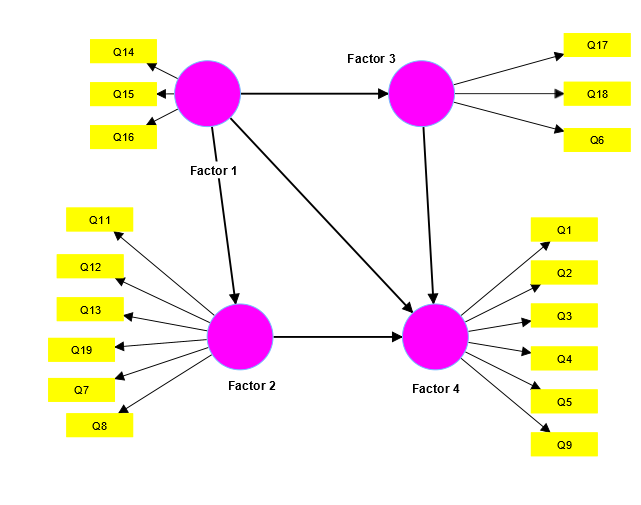
Figure 1.

Modeling Graphics of Reflective Model in SmartPLS

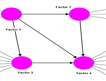
Figure 2.

Structural Part of the Model

Another form of specification of measurement in SEM studies is reflective and formative modeling (see Ghanbar, 2023; Sarstedt et al., 2021). The reflective model (see Figure 1) is grounded in classical test theory (CTT), indicating that each indicator represents the influence of its corresponding latent variable. It should be mentioned that reflective indicators, also known as effect indicators in the psychometric literature, can be seen as a representative subset of all possible items within the conceptual domain of the construct and the construct is the common cause for all of its items. Conversely, formative measurement models (see Figure 3) operate under the assumption that the indicators combine linearly to create the construct. Consequently, this type of measurement model is often referred to as a formative index.

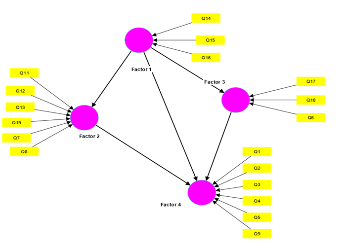
Figure 3.

Formative Constructs in a PLS-SEM Model

As can be seen in Figure 3, in the formative model, the direction of the relationship is reversed. In this model, the indicators cause or form the construct, which is also known as an emergent factor (see also Diamantopoulos & Siguaw, 2006, Hair et al., 2022). In contrast to a reflective model, the indicators in a formative model are not interchangeable, and, hence, removing any of them would result in a loss of meaning for the construct (Diamantopoulos et al., 2008). This loss of meaning also depends on the number of indicators. In the case of subtests in a test, for example, each part must address a distinct aspect of the construct, which AL researchers should establish first. To conclude this section, it should be noted that determining whether to use reflective or formative models SEM depends on several considerations related to the nature of the construct. These criteria are conceptual understanding of the construct, indicator characteristics, theoretical basis, and empirical assessment. It should be noted that this is a controversial topic in the other disciplines; yet in AL, these issues have recently come to the forefront, especially with the results of the latest review on SEM (Rezvani & Ghanbar, 2023), highlighting that formative models are uncommon in SEM studies (see also Hair & Almar, 2022).

3 | Assessing Reflective Measurement Models Using SmartPLS

As it was mentioned before, the use of reflective models in AL is very widespread (see Ghanbar & Rezvani, 2023) and this is due to the fact that the majority of software packages exploited in the field are capable of processing such models. For example, AMOS, one of the most recurrently used software packages in the field, is a covariance-based software and is merely estimating reflectively-framed constructs (see Sarstedt et al., 2021 for a difference between variance-based and covariance-based SEM).

          For validation of reflective measurement models (the relationship between constructs and their related items are evaluated in measurement models, see Figure 1), SmartPLS provides a comprehensive and organized output and this output (see Figure 4) is based on the framework proposed by Hair et al., (2022). Hair et al. (2020) referred to this stage's procedures and assessments as confirmatory composite analysis (CCA). As illustrated in Figure 4, SmartPLS provides a comprehensive and user-friendly graphical output. This unique feature includes a wide range of measures for validating measurement models, which will be the focus of the following discussion.

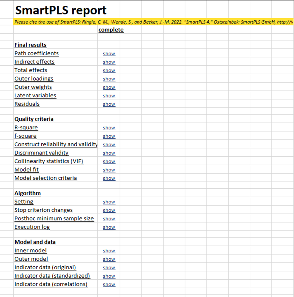
Figure 4.

The Output of SmartPLS for Evaluation of SEM Models

Analyzing PLS-SEM estimates allows researchers to assess the reliability and validity of the construct measures. The first step in evaluating a reflective measurement model is checking the indicator (items of a questionnaire for example) reliability. The term indicator reliability is often used to describe the magnitude of the outer loading. It is essential for all indicators' outer loadings to be statistically significant. However, since a significant outer loading might still be relatively weak, a general guideline is that standardized outer loadings should be at least 0.708. As can be seen in Figure 5, the program automatically flagged outer loadings below 0.708. Although indicators with outer loadings below 0.708 are candidates for removal, the effects of removing an indicator on other reliability and validity measures of the model should be carefully inspected. Typically, indicators with outer loadings ranging from 0.40 to 0.70 should only be considered for removal if doing so enhances internal consistency reliability or convergent validity (see Hair et al., 2020 for other considerations in relation to removing items).

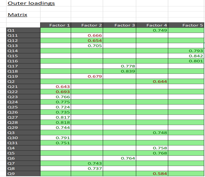
Figure 5.

Outer loadings in SmartPLS

The second step is to assess internal consistency reliability. Cronbach’s alpha is the traditional measure used for evaluating internal consistency, yet it has several drawbacks like sensitivity to the number of items in a questionnaire (see Ghanbar, 2023 for the other limitations in using Cronbach alpha). In PLS-SEM (see Hair & Almar, 2022), indicators are prioritized based on their individual reliabilities and given the inherent limitations of Cronbach’s alpha, it is technically more appropriate to employ composite reliability (CR). CR considers the outer loadings of the indicators (items of factors in questionnaire, for example). As Hair et al., (2022) recommended, CR values between 0.60 and 0.70 are acceptable in the exploratory research (e.g., the initial phases of the validation of a questionnaire, for example), and in more advanced stages values between 0.70 and 0.90 are satisfactory. As can be seen in Figure 6, CR and Cronbach alpha are presented in the output of SmartPLS. It should be mentioned that if each of these reliability measures is below the cut-off recommended values, the program will flag them, a notable and unique feature among other SEM programs, besides a good graphical representation.

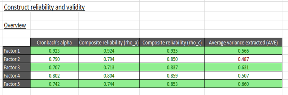
Figure 6.

Reliability Measures in SmartPLS

The third step in validating the reflective measurement model is assessing the convergent validity and variance explained in the model. SmartPLS provides a well-designed and organized graphical output for this step. Convergent validity refers to the degree to which different indicators of the same construct (e.g., one of the factors a questionnaire) align or concur within a measurement model (see Hair et al., 2021). In fact, it assesses the extent to which these indicators share a substantial amount of common variance. A common measure to establish the convergent validity of a construct is the average variance extracted (AVE), defined as the grand mean of the squared loadings of the indicators for a construct which involves summing the squared loadings and then dividing by the number of indicators; thus, AVE is analogous to the communality of a construct. The common rule of thumb is that AVE should be 0.5 or higher (see Hair et al., 2010). Items in a questionnaire with loadings less than .4 should be removed and those with loadings in the range of .4 and .7 should be deleted if their removal results in an increase in AVE and CR values (see the flagged value of AVE in Figure 7 which is less than 0.7), which is why the program represents AVE in accompanying with CR in Figure 6.

          The final step in evaluating a reflective measurement model is examining discriminant validity. Discriminant (or divergent) validity refers to the degree to which a construct is differentiated from other constructs (in a questionnaire, for example) through its specific items or indicators. Therefore, discriminant validity signposts that a construct is unique and encompasses aspects that are not covered by other constructs within the model.

          Different recommendations have been proposed for assessing the discriminant validity. The first criterion is the Fornell-Larcker criterion which states that the square root of each construct’s AVE should be greater than its correlation with any other constructs in the model. This criterion helps ensure that each construct is sufficiently distinct from the others in terms of the variance it explains relative to its measurement error. As can be seen in Figure 7, the program, in a neat and tidy way, yields a table for assessing the tenability of this criterion wherein the square root of each construct’s AVE is presented which can then be compared with the correlation of each construct with another (we in this study take the term “construct” and “factor” equivalent as we mentioned before).

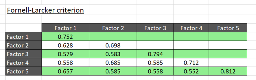
Figure 7.

Square Root of each Construct’s AVE

Another criterion for evaluating discriminant validity is to compare cross loadings. More specifically, the outer loading of each item of a construct (a factor of a questionnaire, for example) should be greater than its outer loadings in other constructs (i.e., cross loadings, see Hair et al., 2022 for more information about cross loadings). As can be seen in Figure 8, this criterion can be meticulously assessed by reading the output of the program.

          Nonetheless, Henseler et al., (2015) demonstrated that cross loadings fail to identify even significant breaches in discriminant validity, making this criterion ineffective for practical research applications. To address this issue, Henseler et al., (2015) recommended using the heterotrait-monotrait ratio (HTMT) of the correlations for a more precise evaluation of discriminant validity. HTMT can be defined as the average of all correlations between indicators from different constructs (heterotrait-heteromethod correlations) relative to the geometric mean of the average correlations between indicators measuring the same construct (monotrait-heteromethod correlations) (see Hair et al., 2022). As suggested by Henseler et al., (2015), a threshold of 0.90 (lower than this value, see Figure 10) for the HTMT metric is acceptable when dealing with path models that encompass constructs of high conceptual similarity. Consequently, an HTMT value surpassing 0.90 implies insufficient discriminant validity. In instances where the constructs within the path model demonstrate a higher degree of conceptual distinctiveness (researchers need to judge this based on the literature and logic), Henseler et al., (2015) suggested a more conservative threshold value of 0.85, thereby ensuring a more rigorous evaluation of discriminant validity. As can be seen in Figure 9, given that all HTMT ratios in the output of SmartPLS are less than 0.85, it can be concluded that discriminant validity is established. It can be concluded that using SmartPLS provides a robust framework for assessing discriminant validity of measurement models which steals a march on other SEM software programs like R or AMOS.

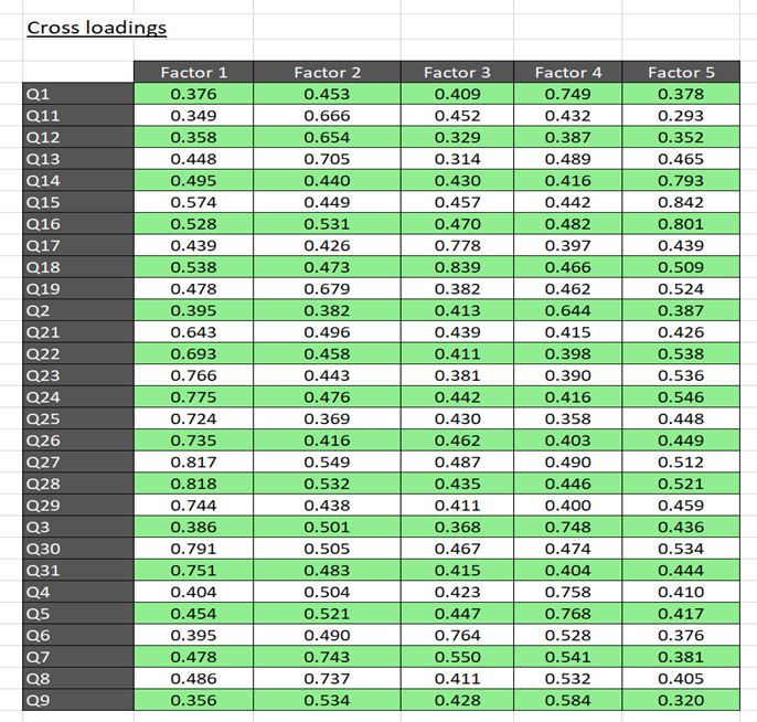
Figure 8.

Cross Loading of Indicators

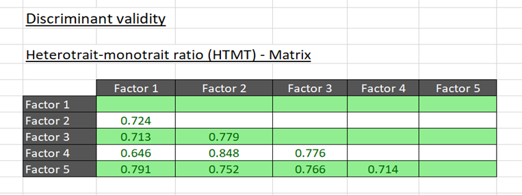
Figure 9.

HTMT Ratios in the Measurement Model

4 | Assessing Formative Measurement Models Using SmartPLS

As mentioned before, the type of relationship between indicators and constructs in the formative measurement models is totally different from what we have seen in the reflective ones, so we need a completely different procedure to evaluate this type of modeling. Here in this type of model, we consider three key phases: a) convergent validity, b) indicators’ collinearity, and c) significance and relevance of the outer loadings. In what follows, the steps relating to each phase will be explained, accompanied by the output from SmartPLS.

          First, to check the convergent validity, we need to check the correlation of the formatively measured construct with the same construct which has a reflective setup (see Figure 10). This type of analysis is called redundancy analysis. Here in this phase, the formatively measured construct will be considered an exogenous latent variable, and the regression weight of the path from this contrast to the reflectively measured one is an indicative of the convergent validity of the formative construct. Based on Hair et al. (2022), the path coefficient between 0.7 and 0.8 or above 0.8 is considered appropriate. One important point which PLS-SEM researcher need to consider is that the reflective construct and its related indicators need to be considered during scale development in accompanying with other constructs which is, in a way, arduous for researchers. It should be noted that Sarstedt et al. (2016) proposed an alternative for this phase which is called global single-item measure and interested readers are referred to this source for more information.

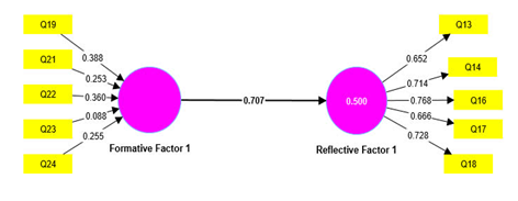
Figure 10.

Redundancy Analysis for Convergent Validity Assessment

The second phase in assessing a formative model is inspecting the model for collinearity issues. As it was mentioned before, indicators in a formative model are unique aspects of a construct, and, hence, should not be highly correlated (see Plonsky & Ghanbar, 2018 for a definition of collinearity of two variables). It should be noted that when there are more than two indicators involved, the situation is referred to as multicollinearity. The reason behind inspecting collinearity is that high levels of collinearity among formative indicators affect both the estimation of weights and their statistical significance. In order to check the collinearity, a variance inflation factor (VIF) measure is proposed (see Plonsky & Ghanbar, 2018 and Ghanbar & Rezvani, 2023 for an elaborated discussion of VIF). It should be noted that without using SmartPLS researcher should first calculate tolerance (TOL), defined as the amount of variance of one formative indicator not represented by the other indicators in the same construct. However, as it is shown in Figure 11, VIF for each indicator in the formative model is calculated and presented by SmartPLS. Normally, VIF values of 5 or more insinuate significant collinearity among the indicators in the formative model. Nevertheless, even lower VIF values like 3 can indicate collinearity issues (Becker, Ringle, Sarstedt, & Völckner, 2015; Mason & Perreault, 1991). Ideally, VIF values should be around 3 or less, as recommended by Hair et al. (2022).

Figure 11.

VIF of Indicators

The third and last phase is testing the significance and relevance of the formative indicators. Here in this phase, we need to test whether the indicators (the items of a construct) truly represent the construct. To achieve this, we need to use the bootstrapping procedure in SmartPLS (see Figure 12) (interested readers are referred to Hair et al., 2022 to become more familiar with the bootstrapping procedure). Before embarking on the evaluation of a formative construct in this part, one note should be mentioned about the number of indicators in a formative construct. When researchers consider a large number of formative indicators to measure a construct, there is an increased likelihood that some indicators will have low or insignificant outer weights. Unlike reflective measurement models, where the number of indicators may not significantly affect measurement outcomes, in a formative measurement there is a ceiling for the maximum number of indicators that can maintain statistically significant weights. More specifically, when indicators are considered uncorrelated, as in a formative construct, the average outer weight is approximately 1 divided by the squared root of the number of indicators. This suggests that by adding more formative indicators to a construct, it is highly likely that some of them will have a non-significant outer weight (see Cenfetelli & Bassellier, 2009 for a strategy in order to deal with these issues in formative constructs).

          As can be seen in Figure 12 and Figure 14, significant indicators have p-values less than 0.05. Nonetheless, not all the indicators which have p-values larger than 0.05 should be deleted. Here in this part and in relation to this, two concepts should be explained.

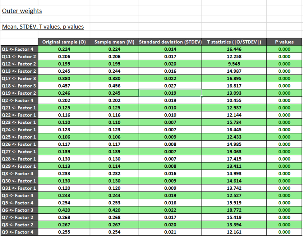
Figure 12.

Tests of Significant Outer Weights of Formative and Reflective Constructs

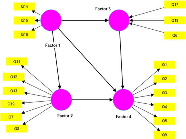
Figure 13.

A Model Comprising Formative and Reflective Constructs

The absolute contribution of an indicator refers to the unique information it provides independently, without accounting for the influence of other indicators related to the formative construct. This absolute contribution is measured by the formative indicator's outer loading, a metric typically reported alongside the indicator's weight. Nonetheless, outer loadings are the regression coefficients of a simple linear regression between indicators and their corresponding construct (see Factor 3 in Figure 13). As a rule of thumb, when an indicator’s outer weight is non-significant, yet its outer loading is high, that is, above 0.50, the indicator should be regarded as absolutely important but not relatively important. Here in this situation the indicator should generally be remained. However, when an indicator's outer weight is non-significant and its outer loading is below 0.50, researchers should evaluate whether to retain or remove the indicator by considering its theoretical significance and any potential content redundancy with other indicators of the same construct. In the last scenario, if an indicator's outer weight is low and its outer loading is below 0.1, it should be removed from the model. As can be seen in Figures 12 and 14, SmartPLS rigorously tested the significance and relevance of formative indicators in all constructs, including construct 3, which is formatively measured. We see that pertaining to Factor 3, (see Figures 12, 13, 14) all indicators (Q17, Q18, Q6) have p values below 0.05, so both their absolute and relative contributions to the construct are significant and they should be remained in the model. 

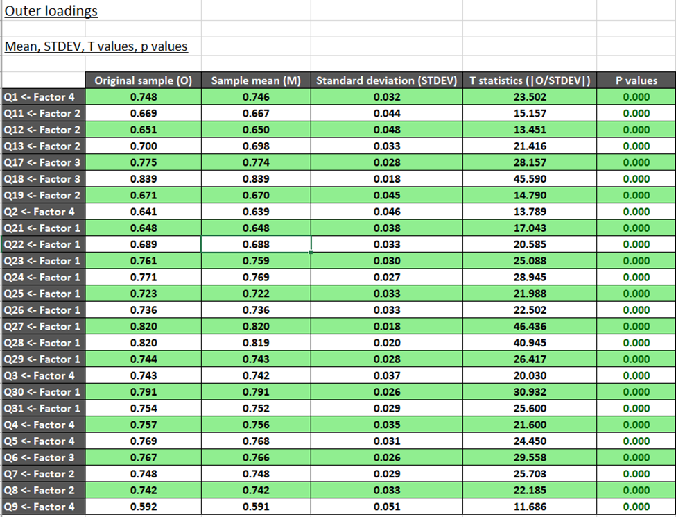
Figure 14.

Tests of Significant Outer Loadings of Formative and Reflective Constructs

5 | Conclusion

In this short method tutorial, attempts have been made to showcase the rigor and versatility of SmartPLS in assessing different types of modeling in measurement models, that is, reflective and formative. Pertaining to reflective models, it was showen that SmartPLS's output is not only neat and tidy graphically, but also it is organized and based on the most recent credible recommendations for assessing the validity of reflective measurement models. Moreover, we illustrated that the program is very versatile in assessing formative models, providing an organized set of outputs to assess a formative model which has less frequently been used in the field of AL and other disciplines in social sciences.

Funding

The author(s) received no specific funding for this work from any funding agencies.

Conflict of Interest

The author(s) declared no potential conflicts of interest with respect to the research, authorship, and/or publication of this article.

Data Availability Statements

The datasets generated during and/or analyzed during the current study are available from the corresponding author on reasonable request.

How to Cite:

Ghanbar, H. (2024). Using SmartPLS for structural equation modeling in applied linguistics: A method note. Educational Methods & Psychometrics, 2:12.

Becker, J. M., Ringle, C. M., Sarstedt, M., & Völckner, F. (2015). How collinearity affects mixture regression results. Marketing Letters, 26, 643–659.  https://doi.org/10.1007/s11002-014-9299-9

Cenfetelli, R. T., & Bassellier, G. (2009). Interpretation of formative measurement in information systems research. MIS Quarterly, 33, 689–708.

Diamantopoulos, A., & Siguaw, J. A. (2006). Formative versus reflective indicators in organizational measure development: A comparison and empirical illustration. British Journal of Management, 17(4), 263–282. https://doi.org/10.1111/j.1467-8551.2006.00500.x

Diamantopoulos, A., Riefler, P., & Roth, K. P. (2008). Advancing formative measurement models. Journal of Business Research, 61(12), 1203–1218. https://doi.org/10.1016/j.jbusres.2008.01.009

Ghanbar, H. (2023). Applying structural equation modeling to second-language (L2) research: Key concepts and fundamental reconsiderations. Journal of English Language Pedagogy and Practice, 16(32), 101–117. https://doi.org/10.30495/jal.2023.1988106.1495

Ghanbar, H., & Rezvani, R. (2023). Structural equation modeling in L2 research: A systematic review. International Journal of Language Testing, 13(Special Issue), 79–108. https://doi.org/10.22034/ijlt.2023.381619.1224

Hair J., & Alamer, A. (2022). Partial Least Squares Structural Equation Modeling (PLS-SEM) in second language and education research: Guidelines using an applied example. Research Methods in Applied Linguistics, 1(3), 100027. https://doi.org/10.1016/j.rmal.2022.100027

Hair J., Howard, M. C., & Nitzl, C. (2020). Assessing measurement model quality in PLS-SEM using confirmatory composite analysis. Journal of Business Research, 109, 101-110. https://doi.org/10.1016/j.jbusres.2019.11.069

Hair, J. F., Astrachan, C. B., Moisescu, O. I., Radomir, L., Sarstedt, M., Vaithilingam, S., & Ringle, C. M. (2021). Executing and interpreting applications of PLS-SEM: Updates for family business researchers. Journal of Family Business Strategy, 12(3), 100392. https://doi.org/10.1016/j.jfbs.2020.100392

Henseler, J., Ringle, C. M., & Sarstedt, M. (2015). A new criterion for assessing discriminant validity in variance-based structural equation modeling. Journal of the Academy of Marketing Science, 43, 115-135. https://doi.org/10.1007/s11747-014-0403-8

Mason, C. H., & Perreault Jr, W. D. (1991). Collinearity, power, and interpretation of multiple regression analysis. Journal of Marketing Research, 28(3), 268–280.

Plonsky, L., & Ghanbar, H. (2018). Multiple regression in L2 research: A methodological synthesis and guide to interpreting R2 values. The Modern Language Journal, 102(4), 713–731. https://doi.org/10.1111/modl.12509

Ravand, H. & Baghaei, P., (2016). Partial least squares structural equation modeling with R. Practical Assessment, Research, and Evaluation, 21(1): 11. https://doi.org/10.7275/d2fa-qv48

Rezvani, R., Ghanbar, H., & Perkins, K. (2024). Considerations and praxis of exploratory factor analysis: Implications for L2 research. Teaching English as a Second Language Quarterly (Formerly Journal of Teaching Language Skills), 43(1), 151–178. https://doi.org/10.22099/tesl.2024.49564.3264

Sarstedt, M., Ringle, C. M., & Hair, J. F. (2021). Partial least squares structural equation modeling. In Handbook of market research (pp. 587–632). Springer International Publishing. https://doi.org/10.1007/978-3-319-05542-8_15-2

Sarstedt, M., Hair, J. F., Ringle, C. M., Thiele, K. O., & Gudergan, S. P. (2016). Estimation issues with PLS and CBSEM: Where the bias lies! Journal of Business Research, 69(10), 3998–4010. https://doi.org/10.1016/j.jbusres.2016.06.007

Tabachnick, B. G., & Fidell, L. S. (2019). Using multivariate statistics (7th Ed.). Pearson.