Full Html
On Specific Objectivity and Measurement by Rasch Models: A Statistical Viewpoint
Full Html
1. Introduction
It is often taken for granted that measurement by Rasch models is characterized by three properties. First, and foremost, that measurement by estimates of person parameters is specific objective; second that measurement by Rasch models is interval scaled; and third that the distribution of measurement error is approximately normal with standard errors of measurement that are without bias and with a standard error that shrinks as the number of items increases towards infinity. This paper will look at these assertions by comparing measurement provided by five different estimators of person parameters in a Rasch model with forty dichotomous items.
Correspondence should be made to Svend Kreiner, Department of Public Health, University of Copenhagen, Denmark. Email: svend.kreiner@mail.tele.dk
© 2025 The Authors. This is an open access article under the CC BY 4.0 license (https://creativecommons.org/licenses/by/4.0/)
1.1 The Outline of the Paper
Section 2 defines the Rasch model and provides a brief overview of some of it is important features, including information on how to estimate the exact distribution of estimates of person parameters in Rasch models. Section 3 describes the way that Rasch (1961) and Rasch (1966) defined the notion of specific objectivity. Section 4 describes and uses different ways to estimate person parameters in Rasch models on the data of a cognitive test with forty dichotomous items. Section 5 examines and compares the biases and the standard errors of measurement provided by the different estimates. This section also assesses the degree to which measurement is interval scaled. Section 6 compares the exact and the asymptotic distributions of the estimates of person parameters. Finally, Section 7 draws conclusions and Section 8 addresses methodological issues.
2. Rasch Models
We refer to Fischer and Molenaar (1995) for comprehensive information on the Rasch model for item analysis. The chapter by Fischer (1995) on the formal aspects of specific objective measurement is particularly important.
2.1 The Rasch Model for Dichotomous Items
We parameterize the Rasch model for dichotomous items in two different ways. Rasch (1961;1966) defined the probabilities of responses to items as a simple multiplicative function of person parameters φv and item parameters di
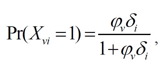
, v = 1,…,n and i= 1,…,k (1)
Today, many prefer an IRT version of the model with θv = ln(φv) and bi=-ln(di) and regard the person parameters θv as outcomes of a latent trait variable T,
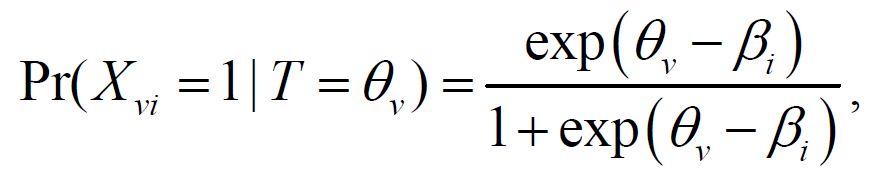
, v = 1,…,n and i= 1,…,k (2)
The two versions are equivalent, and it does not matter whether one uses one or the other during item analysis. However, rewriting (1) as (2) has one important consequence. It posits the Rasch model as a special simple member of the family of IRT models. This is useful, because it means that IRT methodology is applicable in connection with item analysis by Rasch models. Some consider it controversial and misleading to view the Rasch model as a particularly simple IRT model. The view in this paper is that Rasch models for item analysis define the intersection between IRT models and the family of measurement models defined by Rasch (1960).
2.2 Important Properties of Rasch Models
Three features that sets Rasch models apart from IRT models are important for the discussions in this paper. The first is that person and item scores are sufficient for person and item parameters, respectively. The second is that it is possible to define two frames of inference that separate person and item parameters. Finally, the third is that the distribution of person scores Rv is a power series distribution.
The conditional distribution of person v’s responses to items given the person’s score Rv over all items defines the first inference frame. It is
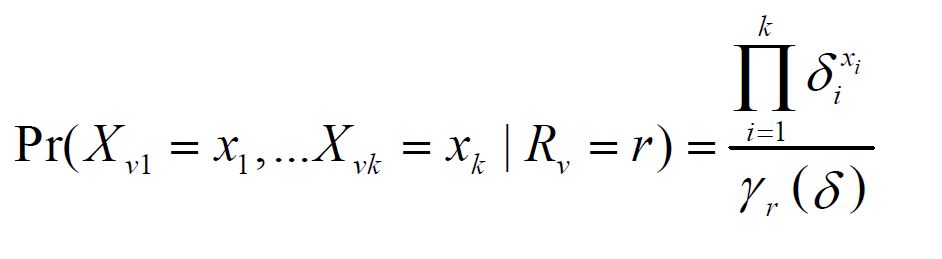 (3)
(3)
where the γr values are symmetrical polynomials of the vector of δ parameters,
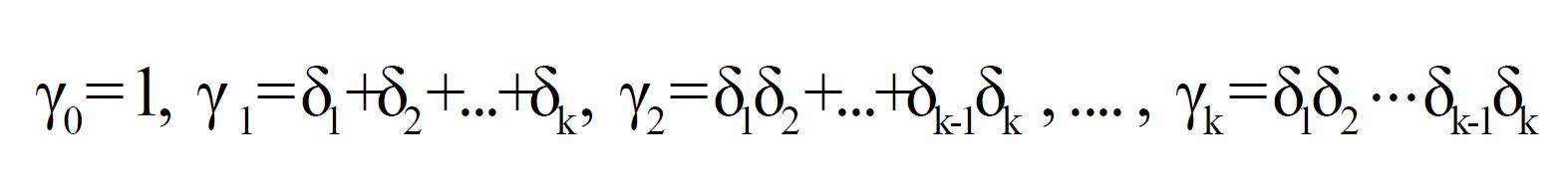
Andersen (1970, 1972, and 1973) derived conditional maximum likelihood estimates (CML) of item parameters and conditional likelihood ratio tests (CLR) of fit of the model within the inference framework defined by (3). These methods illustrate some of the things that Rasch (1961) envisioned when he defined the notions of specific objective measurement and inference.
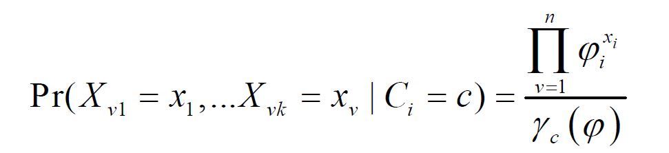
The conditional distribution of responses to item i given the total item score Ci over all persons defines the second inference frame.
 (4)
(4)
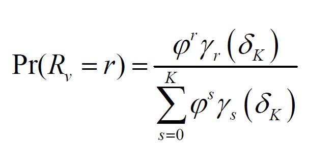
In principle, CML estimation of person parameters should be possible in the framework defined by (4) because the model is symmetrical in item and person parameters. However, inference in the framework defined by (4) was, for technical IT-reasons, a serious challenge in the seventies, and we are not aware of any attempts to implement CML estimates of person parameters until today. We return to this issue in Section 3 on specific objectivity. Finally, the distribution of the total person score is a power series distribution with score parameters that are equal to the symmetrical polynomials of item parameters.
 (5)
(5)
2.3. The Exact Distribution of Estimates of Person Parameters in Rasch Models
The results summarized in Formulas (3) – (5) originated in Rasch (1960). At that time, and quite a few years after that, there were few attempts to estimate the person parameters of the Rasch models. For this reason, nobody was concerned about the distributions of such estimates, and nobody recognized a unique possibility implied by sufficiency and (5) until Kreiner and Christensen (2013) explained how to estimate the distribution of estimates of person parameters in Rasch models. There are two reasons why this is possible.
The first is that the person score is sufficient for the person parameter. From this it follows that likelihood-related estimates of person parameters in Rasch models are defined by monotonic functions of the person score R. The second is that the power series distribution of the person score is known and can be estimated if estimates of item parameters are available.
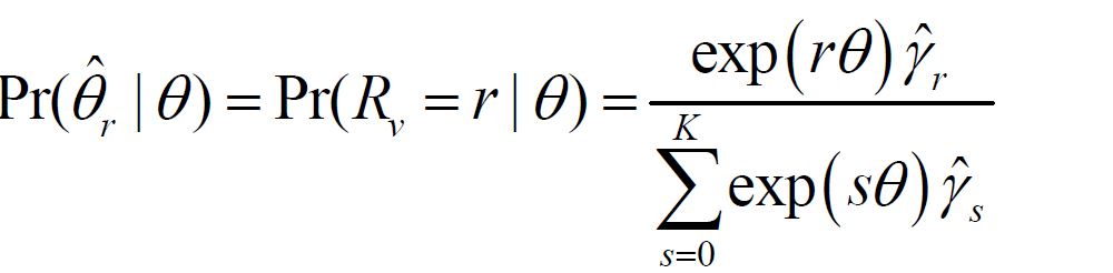
Let = f MLE(r) be the MLE estimate of θ. To estimate the distribution of
, we calculate the symmetrical polynomials of the estimates of the δ parameters and the probabilities of
as shown in Formula (6)
 (6)
(6)
Formula (6) provides the information we need to describe the exact distribution of . It tells us how to estimate the probabilities and how to assess the bias and the standard error of measurement (SEM) of
. Conditionally given a specific value of the person parameter θ, the expected estimate is
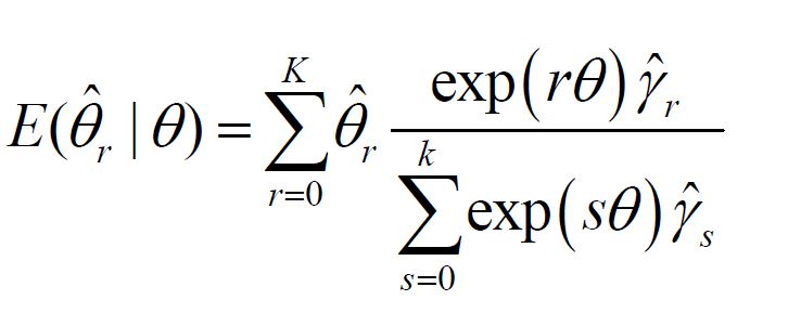 (7)
(7)
The bias of the estimate is
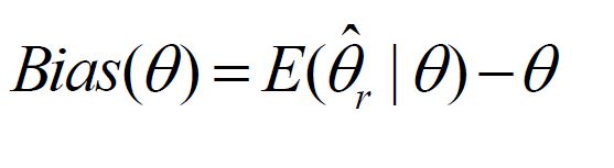 (8)
(8)
Finally, the standard error of measurement (SEM) is defined by the RSME rather than the standard error of the estimate
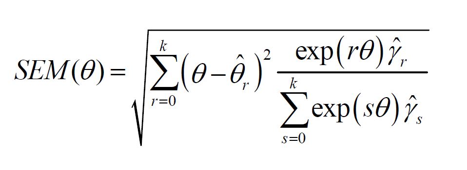 (9)
(9)
3. Specific Objectivity
Think of an educational test consisting of a sample of items from a large item bank and a sample of students that respond to the test. In such situations, we use estimates of person parameters of an IRT or Rasch model as measures of a latent traits or abilities.
The properties summarized in formulas (3) – (5) were derived in the Rasch (1960) monograph on measurement models. Rasch’s notion of specific objective measurement were implied by these results, but the first explicit definition can be found in Rasch (1961 and 1966).
In the 1961 paper, formulas (3.10) and (3.11) correspond to (3) and (4) in this paper. Rasch (1961) summarized the usefulness of these results as follows:
On the basis of (3.10) we may estimate the item parameters independently of the personal parameters, the latter having been replaced by something observable, namely by the individual total number of correct answers. Furthermore, on the bases of (3.11) we may estimate the personal parameters without knowing the item parameters which have been replaced by the total number of correct answers per item. (p. 314)
Rasch does not refer specifically to the notion of specific objectivity in the 1961 paper, but it is apparent that this is where he laid the groundwork. Estimates of item and person parameters in these inference frames are “indispensable for well-defined comparisons of measurements” because:
Comparison between two stimuli should be independent of which particular individuals were instrumental for the comparison; and it should also be independent of which other stimuli within the considered class were or might have been compared. Symmetrically, a comparison between two individuals should be independent of which particular stimuli within the class considered were instrumental for the comparison; and it should also be independent of which other individuals were also compared, on the same or some other occasion. (Rasch, 1961, p. 322)
The above quote encapsulates what many understand about specific objective measurement. However, “specific objectivity” was not coined in the 1961 paper and the requirement of independence is less than precise because “independence” like “invariance” is a generative term.
However, Rasch coined the terminology “specific objectivity” and provided a formal statistical definition in the 1966 paper. During a discussion of the conditional distributions defined by Formulas (3) and (4) of this paper he first pointed out that “we can estimate the person parameters without knowing or simultaneously estimating the item parameters” (Rasch, 1966, p. 23). The insight summarized in this quote is important. It makes it clear what Rasch meant when he talked about separating persons from items and suggested that:
The principle of separability leads to a singular objectivity in statements about both parameters and model structure. In fact, the comparison of any two subjects can be carried out in such a way that no other parameters are involved than those of the two subject – neither the parameter of any other subject nor any of the stimulus parameters. Similarly, any two stimuli can be compared independently of all other parameters than those of the two stimuli, the parameters of all other stimuli as well as the parameters of the subjects having been replaced with observable numbers. It is suggested that comparisons carried out under such circumstances be designated as ´specific objective’. (Rasch, 1966, p. 24–25)
Rasch had used the terminology in lectures and informal notes several years before 1966. However, it was introduced for the first time in a published paper in 1966 together with the mathematical statistical definition summarized below. Rasch’s definition of specific objectivity asserts that:
Measurement of latent traits by estimates of person parameters in Rasch models is specific objective if and only if the estimate does not involve estimates of item parameters and information on measurements of traits of a sample of other persons.
3.1 Measurement of Difficulties of Items
The theory of specific objectivity includes measurement of item difficulties. Christensen (2013) describes three estimates of item parameters in Rasch models, two of which provide specific measurement of item difficulties. The first is the conditional maximum likelihood (CML) estimate of Andersen (1970, 1972); the second is the pairwise conditional estimate (PCE) described by Zwinderman (1995).
There is no doubt that Rasch was thinking about conditional maximum likelihood estimates in the 1961 and 1966 papers. However, the PCE estimates of item parameters shows that different estimators may provide specific objective measurement and that they can do that without reference to the inference frame defined by Formula (3). The PCE therefore raises issues about the quality of the estimators. In this case, the CML and PCE are asymptotically consistent, but Christensen (2013) claim that the PCE is less efficient than the CML, because it relies on a restricted amount of information.
The third estimate of item parameters in Rasch models is the so-called marginal maximum likelihood (MML) estimate. The MML is not specific objective, because it involves estimates of the distribution of person parameters in the study sample, but it is asymptotically consistent. Zwinderman and Wollenberg (1990) maintain that MML estimates of item parameters may be superior to CML estimates if the distribution of the person parameters is correctly specified.
The claims of Zwinderman and Wollenberg raise the issue that this paper intends to address. Is specific objective measurement by CML estimates superior to measurement by estimates of person parameters in Rasch models that do not satisfy Rasch’s requirement of measurement that do not involve estimates of item parameters? To address this issue, we will estimate person parameters of a Rasch model for dichotomous items using both CML estimates and estimates by a number of often used estimators that involve estimates of item parameters.
4. Estimates of Person Parameters in a Rasch Model for Dichotomous Items
We use data from the validation study of a Danish cognitive test referred to as CHIPS (Children’s Problem Solving). CHIPS includes forty dichotomous items and data contains responses to items from three groups of students from the Danish public schools:
- 78 students receiving special education (mean = 19.5, SD = 7.7)
- 454 at Grade 2 (mean = 22.0, SD = 7.5)
- 382 at Grade 5 (mean = 28.1, SD = 5.8)
Figure 1 shows histograms of the person score in the three groups and Appendix A provides information on the estimates of the item and person parameters of the Rasch model. The test of fit of the Rasch model did not disclose evidence of DIF or lack of invariance in different grades.
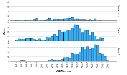
Figure 1.
Distribution of CHIPS Scores at Three Different Grades
In addition to the CML, we may calculate estimates of person parameters by four different estimators. The first of these is the joint maximum likelihood (JML) estimate of items and person parameters proposed by Wright and Panchapakesan (1969). The JML did not satisfy Rasch[1]. However, it was a major accomplishment in 1969, and it was in a sense objective, because it was sample-free and did not need a specific distribution of the sample of persons.
Hoijtink and Boomsma (1995) describe estimates of person parameters in IRT models that can be used to estimate person parameters in Rasch models: the maximum likelihood estimator (MLE) described by Birnbaum (1968) and Lord (1973), the weighted likelihood estimator (WLE) proposed by Warm (1989), the Bayes modal estimator (BME) and the Bayes expected a posteriori estimator (EAP). All these estimators are examples of joint inference because they depend on the CML estimates of item parameters. The MLE and WLE estimators are sample-free, but the BME and EAP are not. They assume that the set of persons responding to items is a random sample from a population with a known distribution of person parameters.
Table 1 provides information on the estimates of person parameters by the CML, JML, MLE and WLE. The Bayesian estimates will be described in Section 6.3. Since CML, JML, and MLE estimates are unavailable for extreme scores, I imputed estimates for these scores in Table 1.
Table 1.
Measurement of Cognitive Level by Estimates of Person Parameters in the Rasch Model for CHIPS
Score | WLE | MLE | CML | JML |
0 | -5,425 | -6,075 | -6,075 | -6,197 |
1 | -4,267 | -4,644 | -4,689 | -4,697 |
2 | -3,695 | -3,891 | -3,935 | -3,942 |
3 | -3,297 | -3,424 | -3,467 | -3,474 |
4 | -2,982 | -3,073 | -3,115 | -3,121 |
5 | -2,716 | -2,784 | -2,826 | -2,831 |
6 | -2,482 | -2,534 | -2,576 | -2,580 |
7 | -2,270 | -2,311 | -2,351 | -2,355 |
8 | -2,073 | -2,106 | -2,145 | -2,148 |
9 | -1,888 | -1,915 | -1,952 | -1,955 |
10 | -1,713 | -1,734 | -1,770 | -1,772 |
11 | -1,544 | -1,561 | -1,595 | -1,596 |
12 | -1,380 | -1,393 | -1,426 | -1,427 |
13 | -1,220 | -1,231 | -1,261 | -1,262 |
14 | -1,064 | -1,072 | -1,100 | -1,100 |
15 | -,909 | -,915 | -,941 | -,941 |
16 | -,757 | -,760 | -,784 | -,784 |
17 | -,605 | -,607 | -,628 | -,628 |
18 | -,454 | -,453 | -,473 | -,472 |
19 | -,302 | -,300 | -,317 | -,316 |
20 | -,150 | -,146 | -,160 | -,159 |
21 | ,003 | ,009 | -,002 | -,001 |
22 | ,158 | ,166 | ,157 | ,159 |
23 | ,316 | ,325 | ,320 | ,322 |
24 | ,476 | ,488 | ,486 | ,488 |
25 | ,640 | ,655 | ,656 | ,658 |
26 | ,810 | ,827 | ,831 | ,834 |
27 | ,985 | 1,006 | 1,013 | 1,016 |
28 | 1,167 | 1,192 | 1,203 | 1,206 |
29 | 1,359 | 1,387 | 1,402 | 1,405 |
30 | 1,561 | 1,594 | 1,614 | 1,617 |
31 | 1,777 | 1,816 | 1,840 | 1,844 |
32 | 2,010 | 2,056 | 2,086 | 2,090 |
33 | 2,265 | 2,320 | 2,357 | 2,361 |
34 | 2,551 | 2,616 | 2,660 | 2,665 |
35 | 2,876 | 2,954 | 3,008 | 3,013 |
36 | 3,256 | 3,351 | 3,417 | 3,423 |
37 | 3,716 | 3,833 | 3,914 | 3,922 |
38 | 4,286 | 4,453 | 4,549 | 4,560 |
39 | 5,042 | 5,373 | 5,373 | 5,260 |
40 | 6,382 | 6,929 | 6,929 | 6,760 |
Note. Imputed estimates are for scores 0 and 40.
Figures 2 to 4 show the distributions of differences between the CML and the other estimates excluding estimates associated with imputed scores to present a fairer picture of the similarity of the estimates.
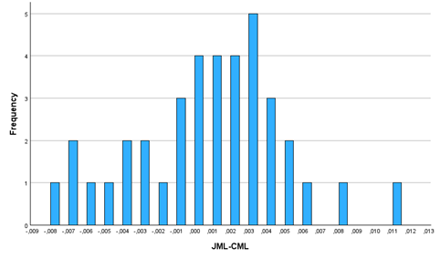
Figure 2.
Differences between CML and JML Excluding Estimates by Extreme Scores
Mean = -0.002
Figure 2 excludes the difference between the CML and JML estimates defined by the person score equal to 39. Apart from that, there is virtually no difference between the conditional and joint maximum likelihood estimates of person parameters. The result is surprising because JML estimates of item parameters are known to be asymptotically inconsistent as the number of persons increase towards infinity. Molenaar (1995, p. 43) claims that “most researchers tend to avoid JML estimation” because of the drawbacks and provide references supporting these claims. However, the discussion of these problems has previously focused on estimation of item parameters and treated person parameters as incidental parameters and little has been said about the asymptotic properties of estimates of person parameters. If it should happen that JML estimates of person parameters are inconsistent as the number of items increases towards infinity, the similarities between the JML and CML estimates in Table 1 and Figure 2 imply that CML estimates of person parameters have the same problem.
Figures 3 and 4 describe the differences between the CML and respectively the MLE and the WLE. Differences are more pronounced than for the JML. In addition to this, it is of some interest that the distribution of differences is skewed for the MLE and symmetric for the WLE. This suggests that the eventual bias of CML estimates may differ systematically from the bias of the MLE.
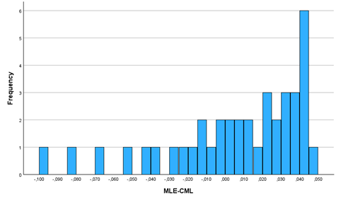
Figure 3.
Differences between CML and MLE Excluding Estimates by Extreme Scores
Mean = 0.005
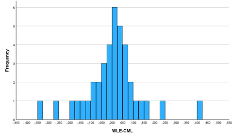
Figure 4.
Differences between WLE and CML Estimates by Extreme Scores
Mean = 0.003
5. Comparison of Estimators from a Statistical Point of View
This section compares the exact distributions of the estimates of person parameters from a statistical point of view. Estimation of parameters in Rasch models must satisfy the same requirements that estimates of parameters in other statistical and probabilistic models have to comply with:
- Measurement should be ratio or interval scaled to facilitate quantitative comparisons.
- Measurement bias must be ignorable.
- Measurement error should be as small as possible even if it is unavoidable.
- The distribution of the estimators must be available to calculate confidence intervals around the estimates.
Obviously, systematic measurement bias is a challenge to objective comparisons of measurements, but it is usually taken for granted that measurement by Rasch models satisfies all the above requirements. Measurement is unbiased because it is known that all of the above estimators – except perhaps for the JML - are asymptotically normal with bias and error that disappears as the number of items increases towards infinity. However, Warm (1989) claims that the advantage of the WLE estimator is that the bias of the WLE is smaller than the bias of the other estimators and therefore acknowledges that bias is an issue. Hoijtink and Boomsma (1995) are also concerned with the application of asymptotic results in cases with few items. They assess the claims of no bias in two simulation studies that confirm that one should not trust asymptotic claims in cases where the number of items is between five and fifteen.
Simulation studies like those presented by Hoijtink and Boomsma (1995) are useful, and they are probably the only way to address asymptotic issues in connection with IRT models. With Rasch models, there is a better way. We use formulas (6) – (8) to calculate estimates of the exact distribution of estimators of person parameters. The imputed values of the CML, JML and MLE are not completely arbitrary, but they do add an element to the calculations that may influence assessment of measurement bias and error.
5.1 Comparison of CML, JML, MLE, and WLE Estimates of Person Parameters
Figure 5 compares the bias and the standard error of measurement (SEM) of the CML and the JML for values of the person parameter θ from -5.0 to +5.0.
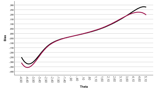
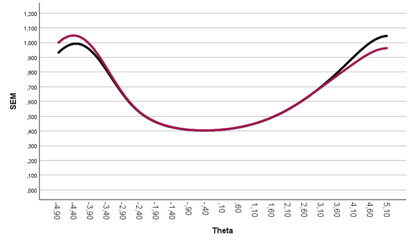
Figure 5.
Comparison of Bias and Standard Errors of CML (Black) and JML (Red) Estimates
There is close to no difference between the two estimates. The ranges of θ values where the absolute bias is below 0.05 is θ Î [-1.45, 1.45] for the CML and θ Î [-1.45, 1.35] for the JML, whereas the SEMs of the CML and the JML is below 0.45 for θ Î [-1.70, 1.05] and θ Î [-1.80, 1.05], respectively. At extreme values, it appears as if the JML performs a little better than the CML. However, we assume that this is probably due to the arbitrary estimates that we imputed for extreme values of the person scores.
Figure 6 compares CML and the MLE. The MLE appears to perform a little better than the CML. The absolute bias of the MLE is below 0.05 for θ Î [-2.30, 2.00] and the SEM is below 0.45 for θ Î [-1.85, 1.20].
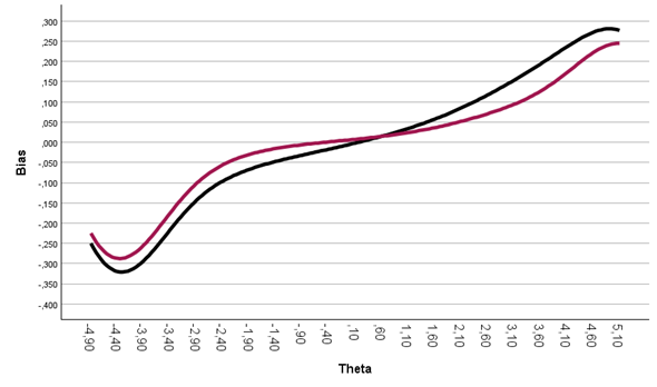
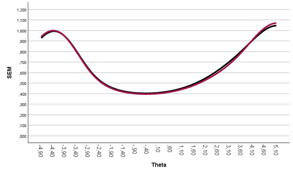
Figure 6.
Comparison of Bias and Standard Errors of CML (Black) and MLE (Red) Estimates
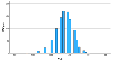
Finally, Figure 7 compares the CML and the WLE. In terms of bias, the difference is dramatic. The absolute bias of the WLE is less than 0.05 for θ Î [-4.10, 4.90] and the SEM is a little better.
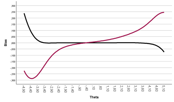
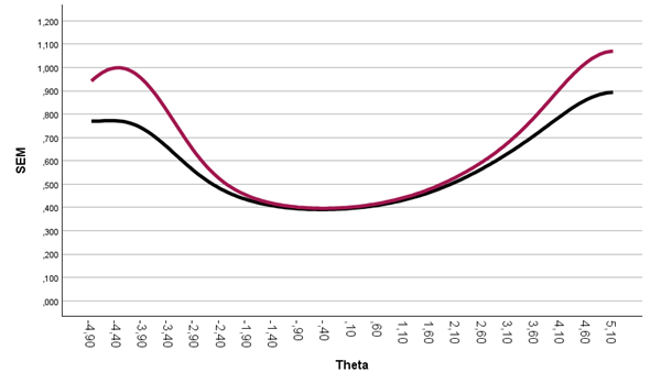
Figure 7.
Comparison of Bias and Standard Errors of WLE (Black) and CML (Red) Estimates
Given these results, three conclusions are unavoidable. The first is that JML is better than its reputation. There is no difference between the performances of CML and JML. Adhering to the rules defined by specific objectivity does not produce better and more adequate measurement than joint maximum likelihood estimation. The second is that the performance of IRT-based estimators of person parameters are superior to the estimates derived specifically for Rasch models. And finally, the third is that WLE estimates clearly outperform the other options and, therefore, WLE should be the default estimator in both Rasch and IRT models. We return to the implication of these results for Rasch’s notion of specific objectivity in the discussion.
5.2 Interval Scaled Measurement?
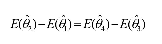
In Rasch models, the person parameters have values on scales with arbitrary origins that the theory of Rasch models refers to as logit scales. It is often claimed that measurement by Rasch models is interval scaled because differences between person parameters are the same on all possible logit scales. However, there is a problem.
To see the problem, consider a situation where differences defined by two pairs of parameters are the same, θ2 – θ1 = θ4 – θ3. The problem is that we do not know the true values of the parameters and therefore must make do with estimates of persons with errors and (possibly) bias. To claim that measurement is interval scaled, we refer to the expected differences between estimates and say that measurement is interval scaled if the estimates of person parameters are unbiased, so that differences between the expected values of estimates are the same as the differences between the person parameters
 (10)
(10)
Table 2 compares the MLE and WML estimates of differences between pairs of person parameters with equivalent differences equal to 2 logits. The table suggests that measurement by the WLE is essentially interval scaled except in two circumstances with extreme cases, whereas we can only say that measurement by the MLE is almost interval scaled relatively close to the origin of the scale.
Table 2.
Estimates of the Lengths of Intervals on the Rasch Models Logit Scale
Score | MLE | WLE | ||
θ1 | θ2 | E(R2)- E(R1) | E( | E( |
-4.5 | -2.5 | 5.0 | 2.221 | 2.111 |
-3.5 | -1.5 | 8.6 | 2.134 | 1.999 |
-2.5 | -0.5 | 11.6 | 2.063 | 2.000 |
-1.5 | 0.5 | 12.7 | 2.031 | 2.000 |
-0.5 | 1.5 | 11.9 | 2.033 | 2.000 |
0.5 | 2.5 | 9.5 | 2.052 | 2.001 |
1.5 | 3.5 | 6.7 | 2.086 | 1.990 |
2.5 | 4.5 | 4.5 | 2.147 | 1.971 |
Table 2 shows that we cannot in general claim that measurement by estimates of person parameters is interval scaled, because the estimates may be biased. Figures 5 – 7 showed that all the estimates that we have considered are close to unbiased within intervals around the origin of the logit scale. The interesting question is how broad these intervals are.
Table 3 provides the answer. The table distinguishes between ignorable and acceptable bias and also shows the range of person parameters where SEMs are less than 0.45. It underscores the conclusion that the WLE is superior to the other estimates, but also points out that there are limits outside which measurement by the WLE is less than precise interval scaled measurement.
Table 3.
Ranges of Person Parameters
Person parameter range | |||
Estimator | |Bias| ≤ 0.01 | |Bias| ≤ 0.05 | SEM ≤ 0.45 |
CML | -0.15 < θ < 0.45 | -1.45 < θ < 1.45 | -1.80 < θ < 1.05 |
JML | -0.20 < θ < 0.40 | -1.45 < θ < 1.35 | -1.80 < θ < 1.05 |
MLE | -1.15 < θ < 1.45 | -2.30 < θ < 2.05 | -1.90 < θ < 1.20 |
WLE | -3.75 < θ < 4.20 | -4.15 < θ < 4.90 | -2.10 < θ < 1.35 |
Note. Ranges of person parameters where measurement bias is ignorable and acceptable and where standard errors of measurement is less than 0.45
5.3 Bayesian Estimates
The JML, MLE and WLE broke the rules of specific objectivity by involving estimates of item parameters. The Bayesian estimates break one more rule by involving estimates of the distribution of the person parameters during estimation of the person parameters. In this subsection, we examine the effect of this on the performance of the Bayes modal estimator (BME).
The BME estimator described by Hoijtink and Boomsma (1995) assumes that the distribution of the person parameter estimates is normal and that estimates of the mean and standard deviation of the distribution are available. Given this information together with estimates of item parameters, the BME estimates the posterior distribution of the person parameters and defines the BME as the modal of this distribution.
Figure 1 showed the distributions of the CHIPS scores in the three groups of students with very different distributions. Table 4 shows the estimates of estimates of the means and standard deviations of the four populations. The BME estimates will routinely assume – without tests of fit - that the distributions of person parameters in the four samples are normal and therefor disregarding that the total sample is a mixture of three subsamples with different distributions.
Table 4.
Estimation of the Means and SD of Normal Distribution of Person Parameters
Grade | Mean | SD |
Special educ. | -0.176 | 1.245 |
Grade 2 | 0.219 | 1.211 |
Grade 5 | 1.369 | 1.090 |
Total | 0.664 | 1.314 |
Table 5 shows the four different BME estimates. It includes the estimates for all the students in the CHIPS study along with those for the students receiving special education, Grade 2 students, and Grade 5 students.
Table 5.
WLE and BME Estimates
BME Estimates | |||||
Score | WLE | All | Spec.educ | Grade 2 | Grade 5 |
0 | -5.425 | -3.640 | -3.720 | -3.600 | -3.160 |
1 | -4.267 | -3.320 | -3.400 | -3.280 | -2.880 |
2 | -3.695 | -3.040 | -3.120 | -3.000 | -2.680 |
3 | -3.297 | -2.800 | -2.840 | -2.760 | -2.480 |
4 | -2.982 | -2.560 | -2.640 | -2.560 | -2.280 |
5 | -2.716 | -2.360 | -2.440 | -2.360 | -2.120 |
6 | -2.482 | -2.160 | -2.240 | -2.160 | -1.960 |
7 | -2.270 | -2.000 | -2.080 | -2.000 | -1.800 |
8 | -2.073 | -1.840 | -1.880 | -1.840 | -1.640 |
9 | -1.888 | -1.680 | -1.720 | -1.680 | -1.480 |
10 | -1.713 | -1.520 | -1.560 | -1.520 | -1.360 |
11 | -1.544 | -1.360 | -1.440 | -1.360 | -1.200 |
12 | -1.380 | -1.200 | -1.280 | -1.240 | -1.080 |
13 | -1.220 | -1.080 | -1.120 | -1.080 | -.920 |
14 | -1.064 | -.920 | -1.000 | -.960 | -.800 |
15 | -.909 | -.800 | -.840 | -.800 | -.640 |
16 | -.757 | -.640 | -.720 | -.680 | -.520 |
17 | -.605 | -.520 | -.560 | -.520 | -.400 |
18 | -.454 | -.360 | -.440 | -.400 | -.240 |
19 | -.302 | -.200 | -.280 | -.240 | -.120 |
20 | -.150 | -.080 | -.160 | -.120 | .040 |
21 | .003 | .080 | .000 | .040 | .160 |
22 | .158 | .200 | .120 | .160 | .320 |
23 | .316 | .360 | .280 | .320 | .440 |
24 | .476 | .520 | .440 | .480 | .600 |
25 | .640 | .640 | .560 | .600 | .760 |
26 | .810 | .800 | .720 | .760 | .880 |
27 | .985 | .960 | .880 | .920 | 1.040 |
28 | 1.167 | 1.160 | 1.040 | 1.080 | 1.200 |
29 | 1.359 | 1.320 | 1.200 | 1.240 | 1.400 |
30 | 1.561 | 1.480 | 1.400 | 1.440 | 1.560 |
31 | 1.777 | 1.680 | 1.560 | 1.600 | 1.760 |
32 | 2.010 | 1.880 | 1.760 | 1.800 | 1.920 |
33 | 2.265 | 2.120 | 1.960 | 2.000 | 2.160 |
34 | 2.551 | 2.320 | 2.160 | 2.240 | 2.360 |
35 | 2.876 | 2.600 | 2.400 | 2.440 | 2.600 |
36 | 3.256 | 2.840 | 2.680 | 2.720 | 2.840 |
37 | 3.716 | 3.160 | 2.960 | 3.000 | 3.160 |
38 | 4.286 | 3.520 | 3.240 | 3.320 | 3.440 |
39 | 5.042 | 3.920 | 3.600 | 3.640 | 3.800 |
40 | 6.382 | 4.360 | 4.000 | 4.040 | 4.200 |
Table 5 illustrates one of the issues that Rasch was concerned with. Consider for instance a student with a total score of 16. If she is receiving special education, the BME estimate is . If she is from Grade 2, it is
. And if she is from Grade 5, the estimate is
. The different estimates provide statements concerning cognitive level that in addition to the total CHIPS score depend on different samples of students. Statements that we would not describe as objective.
Notice also that the unbiased WLE estimates are less than the BME estimates defined by the complete sample of students for scores below 25 and larger for scores above 25, thus indicating the same kind of bias of the BME that we have seen for other estimates. Whether this is because the distribution of the person parameters cannot be normal, we cannot say. Another interesting point is that the narrow [0.70, 0.85] range of person parameters where the bias of BME is ignorable does not include the origin of the logit scale. This is different from the other estimates of person parameters that we have looked at in this paper. Addressing these issues may be interesting but would be a waste of time. Bayesian estimates are not objective and should not be used to provide measurement by Rasch models.
6. Exact or Asymptotic Distributions?
We need the distributions of estimates of person parameters if we want to calculate confidence intervals around measures of traits and they may also be useful in connection with tests of fit of the model and tests of differences between estimates. In principle, this should not be a problem. In practice, the situation is different. Kreiner and Christensen (2013) described the exact distributions of estimators of person parameters in Rasch models and calculation of estimates of the probabilities is no challenge. Estimates of exact distributions of the estimators of person parameters are, however, not available in the large majority of IT-applications that support item analysis by Rasch models and users of these programs have to rely on asymptotic approximations that require the number of items to increase towards infinity.
Hoijtink and Boomsma (1995) describe the asymptotic distributions. All the estimators discussed in this paper, including the BME, are asymptotically equivalent. Measurement bias disappears, the asymptotic distribution of the estimates is normal with decreasing standard deviations and the calculation of confidence intervals around the estimates is straightforward. However, the number of items is usually far from infinite. In terms of the number of items, estimating person parameters in Rasch models is a small-sample exercise where we cannot automatically rely on asymptotic results.
Hoijtink and Boomsma (1995) addressed this issue by simulation experiments with 5, 15 and 25 items. They concluded that there are considerable differences between the properties of the estimators in finite samples and that the distributions of the MLE and WLE are non-normal in cases with 25 items. In this section we will compare the exact and asymptotic distributions of WLE estimates in CHIPS to see whether fifteen additional items fix their discouraging conclusions.
Tables 6 and 7 show the exact probability distributions of person scores and WLE estimates anchored at 11 person parameter values from θ = -5.0 to θ = 5.0. We already know that the distributions are discrete with a range of 41 logit values. However, to emphasize the discrete nature of the distributions, the tables do not show probabilities less than 0.0000005.
The distribution anchored at θ = 0.0 appears in both tables. At this point, the distribution is similar to a discrete distribution with a range of 25 different logit values. Since skewness is close to zero at this point, an approximation by a normal distribution may be conceivable. However, the skewness increases as θ decreases towards -5.0 and increases towards 5.0, and the number of values that we expect to see in practice decreases to a point where approximations by a normal distribution is unrealistic.
Assume that we are satisfied with the asymptotic distribution anchored at the origin of the logit scale and dissatisfied at the extreme ends. The degree to which this is a problem, in practice depends on the location of the persons. The distribution of the WLE estimates for the 914 students in the CHIPS study can be seen in the Appendix. 93 % of the students had estimates of person parameters within the [-2,2] interval: 18 % with estimates below and 75 % with estimates above zero. If the approximations by the asymptotic normal distributions appear to be adequate within the [-2,2] interval and if the exact confidences defined by conventional 95 % confidence intervals are the same, we will conclude that the asymptotic results are applicable in connection with CHIPS.
To assess this, Tables 6 and 7 and Figure 8 display the histograms of the distributions of the WLE estimates for θ equal to -2, 0 and 2 and Table 8 summarizes information on confidence intervals defined by the distributions in Tables 6 and 7.
Table 6.
Exact Distribution of the WLE Estimate for Six Values of θ
Person parameter and expected person score R | |||||||
Θ = -5 | Θ = -4 | Θ = -3 | Θ = -2 | Θ = -1 | Θ = 0 | ||
Score | WLE | R=0.7 | R=1.8 | R=4.2 | R=8.5 | R=14,5 | R=20.2 |
0 | -5.425 | .483073 | .147756 | .008264 | .000016 | ||
1 | -4.267 | .358912 | .298412 | .045369 | .000243 | ||
2 | -3.695 | .125629 | .283930 | .117340 | .001708 | ||
3 | -3.297 | .027579 | .169430 | .190335 | .007533 | .000002 | |
4 | -2.982 | .004264 | .071216 | .217471 | .023395 | .000014 | |
5 | -2.716 | .000495 | .022451 | .186359 | .054496 | .000090 | |
6 | -2.482 | .000045 | .005519 | .124533 | .098990 | .000444 | |
7 | -2.270 | .000003 | .001086 | .066618 | .143943 | .001755 | |
8 | -2.073 | .000174 | .029063 | .170699 | .005658 | ||
9 | -1.888 | .000023 | .010482 | .167352 | .015078 | .000003 | |
10 | -1.713 | .000003 | .003158 | .137039 | .033562 | .000015 | |
11 | -1.544 | .000801 | .094463 | .062887 | .000078 | ||
12 | -1.380 | .000172 | .055143 | .099790 | .000335 | ||
13 | -1.220 | .000031 | .027387 | .134720 | .001229 | ||
14 | -1.064 | .000005 | .011613 | .155285 | .003851 | ||
15 | -.909 | .000001 | .004216 | .153227 | .010328 | ||
16 | -.757 | .001313 | .129681 | .023760 | |||
17 | -.605 | .000351 | .094256 | .046944 | |||
18 | -.454 | .000081 | .058876 | .079709 | |||
19 | -.302 | .000016 | .031611 | .116331 | |||
20 | -.150 | .000003 | .014583 | .145878 | |||
21 | .003 | .005775 | .157034 | ||||
22 | .158 | .001960 | .144902 | ||||
23 | .316 | .000569 | .114376 | ||||
24 | .476 | .000141 | .077016 | ||||
25 | .640 | .000030 | .044086 | ||||
26 | .810 | .000005 | .021360 | ||||
27 | .985 | .000001 | .008713 | ||||
28 | 1.167 | .002973 | |||||
29 | 1.359 | .000841 | |||||
30 | 1.561 | .000196 | |||||
31 | 1.777 | .000037 | |||||
32 | 2.010 | .000006 | |||||
33 | 2.265 | .000001 | |||||
Mean | -4.721 | -3.972 | -3.002 | -2.000 | -1.000 | .000 | |
SD | .771 | .748 | .569 | .439 | .396 | .395 | |
Skewness | 1.225 | -0.520 | -0.862 | -0.318 | -0.073 | .062 | |
Note. Green cells indicate the modes of the distributions
Table 7.
The Exact Distribution of the WLE Estimate for Six Values of θ
Person parameter and expected person score R | |||||||
Θ = 0 | Θ = 1 | Θ = 2 | Θ = 3 | Θ = 4 | Θ = 5 | ||
Score | WLE | R=20.2 | R=27.0 | R=31.8 | R=35.1 | R=37.3 | R=38.7 |
9 | -1.888 | .000003 | |||||
10 | -1.713 | .000015 | |||||
11 | -1.544 | .000078 | |||||
12 | -1.380 | .000335 | |||||
13 | -1.220 | .001229 | |||||
14 | -1.064 | .003851 | |||||
15 | -.909 | .010328 | .000001 | ||||
16 | -.757 | .023760 | .000008 | ||||
17 | -.605 | .046944 | .000041 | ||||
18 | -.454 | .079709 | .000191 | ||||
19 | -.302 | .116331 | .000759 | ||||
20 | -.150 | .145878 | .002586 | ||||
21 | .003 | .157034 | .007568 | .000002 | |||
22 | .158 | .144902 | .018983 | .000011 | |||
23 | .316 | .114376 | .040730 | .000062 | |||
24 | .476 | .077016 | .074550 | .000307 | |||
25 | .640 | .044086 | .116001 | .001298 | |||
26 | .810 | .021360 | .152778 | .004648 | .000002 | ||
27 | .985 | .008713 | .169401 | .014008 | .000020 | ||
28 | 1.167 | .002973 | .157102 | .035313 | .000135 | ||
29 | 1.359 | .000841 | .120885 | .073861 | .000769 | .000001 | |
30 | 1.561 | .000196 | .076422 | .126928 | .003592 | .000007 | |
31 | 1.777 | .000037 | .039212 | .177031 | .013618 | .000068 | |
32 | 2.010 | .000006 | .016081 | .197355 | .041266 | .000564 | .000001 |
33 | 2.265 | .000001 | .005169 | .172452 | .098018 | .003643 | .000024 |
34 | 2.551 | .001270 | .115136 | .177887 | .017969 | .000318 | |
35 | 2.876 | .000230 | .056750 | .238340 | .065446 | .003145 | |
36 | 3.256 | .000029 | .019692 | .224804 | .167797 | .021917 | |
37 | 3.716 | .000002 | .004494 | .139449 | .282937 | .100455 | |
38 | 4.286 | .000611 | .051526 | .284181 | .274266 | ||
39 | 5.042 | .000043 | .009842 | .147549 | .387087 | ||
40 | 6.382 | .000001 | .000732 | .029839 | .212787 | ||
Mean | .000 | 1.000 | 2.000 | 3.001 | 3.994 | 4.940 | |
s.d. | .395 | .427 | .501 | .620 | .776 | .892 | |
Skewness | .062 | .209 | .406 | .592 | .705 | .138 | |
Note. Green cells indicate the modes of the distributions.
θ = -2.0
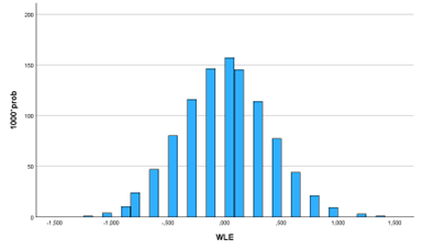
θ = 0.0
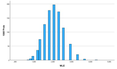
θ = 2.0
Figure 8.
Histograms of the WLE Distributions Anchored at Three Values of θ
Figure 8 shows three histograms of distributions that are close to symmetrical and may appear normal. However, we remind the reader that the distributions are discrete with ranges of outcomes that only include the 20 – 25 values that we would expect to see in practice. We leave it to the reader to decide whether they, in general, would be comfortable with approximation of such variables by normal distributions. However, if we only intend to use the normal approximation to construct confidence intervals around WLE estimates, Table 8 shows that there is little to be concerned about. Table 8 includes information on the exact confidence of the intervals defined by the asymptotic distribution by summarizing the probabilities of WLE estimates below and above the intervals. The probabilities of WLE values below and above the interval are not symmetrical, but the exact confidence defined by the interval is very close to the 95 % that we have asked for. For this specific purpose, the normal approximation is therefore more than adequate for θ values within the [-2.0, 2.0] interval.
Table 8.
Summary of Information on the Distributions of WLE Estimates
θ | Outcomes with probability ≥ 0.000005 | Mean ± 1.96×sd | Probabilities below and above interval | Confidence | |
-5.0 | 8 | [-6.232,-3.210] | .0000 | .0048 | 99.5 % |
-4.0 | 11 | [-5.438,-2.506] | .0000 | .0068 | 99.3 % |
-3.0 | 16 | [-4.117,-1.887] | .0536 | .0042 | 94.2 % |
-2.0 | 21 | [-2.860,-1.140] | .0329 | .0176 | 94.9 % |
-1.0 | 25 | [-1.776,-0.224] | .0230 | .0231 | 95.3 % |
0.0 | 25 | [-0.770,0,770] | .0158 | .0341 | 95.0 % |
1.0 | 23 | [0.165,1.835] | .0301 | .0228 | 94.7 % |
2.0 | 20 | [1.018,2.982] | .0203 | .0248 | 95.5 % |
3.0 | 15 | [1.777,4.223] | .0181 | .0621 | 91.9 % |
4.0 | 12 | [2.475,5.525] | .0043 | .0298 | 96.6 % |
5.0 | 9 | [3.200,6.684] | .0065 | .0000 | 99.4 % |
7. Conclusions
The results in this paper support the following conclusions.
- CML estimates are not the superior estimates. There is no difference between CML and JML, and the MLE performs a little better than the CML.
- WLE is the superior estimate. It is virtually unbiased except for extreme values of θ.
- Bayesian estimates illustrate what Rasch was concerned with when he coined the notion of specific objectivity. Bayesian estimates involve estimates of the parameters of the distribution of persons which generates bias and makes it impossible to compare estimates of person parameters from different populations and samples.
- In CHIPS, measurement by the WLE is interval scaled from -3.8 to 4.2 and essentially interval scaled from -4.2 to 4.9. In many similar realistic settings, measurement will be interval scaled for the majority of the persons responding to items.
- The exact distribution of estimates of person parameters is discrete with a limited number of outcomes. Approximations by normal asymptotic distribution are doubtful, but the approximation may, depending on the population, be adequate and useful for the calculation of confidence intervals around WLE estimates defined by responses to more than 40 dichotomous items.
8. Discussion
8.1 Specific Objective Measurement
The author of this paper admits to an orthodox reading of the canonical scriptures by Rasch (1960, 1961, 1966)[2], and quietly wonders why many advocates of Rasch measurement ignore that estimates of person parameters do not provide specific objective measurement if estimates of item parameters are involved.
However, the results of this paper and several similar experiences have been eye-opening and the view today is rather agnostic. The CML estimate of person parameters in Rasch models does not support the claim that specific measurement is superior and more objective than measurement by all other estimators of person parameters in Rasch models. For now, that prize has to go to the WLE. On the other hand, the WLE illustrates that it is possible to reduce the bias of the MLE. Because of this, and because there are ways to improve the WLE in Rasch models[3], we do not rule out that it may be possible to improve the CML estimate and that an estimator with less bias and smaller SEMs than the WLE may turn up.
8.2 Essentially Objective Measurement
Until a virtually unbiased estimator that does not involve estimates of item parameters is available, we have to reconsider Rasch’s insistence on specific objectivity. Specific objective measurement of cognitive level by the CML is possible in CHIPS, but measurement is biased to a degree, where we cannot claim that we have interval-scaled measurement. Compared to this, measurement by the WLE is virtually without bias and more precise than measurement by the CML. From a statistical point of view, the WLE may not be specific objective, but it is clearly superior to the CML and, therefore, has to be the prefered measure.
Rasch (1967) described a situation where he stressed that it is important that measurement is unbiased. During attempts to estimate scoring functions of Rasch’s original model for polytomous items, it turned out to be impossible to separate person, item and category scores in the same way as for the dichotomous items. However, Rasch remarked that they could obtain some sort of “unbiased estimates” where the precision depended on the other parameters. He pointed out that “the estimation cannot be specifically objective”, but also that “this conjecture points to a possible relaxation of our basic concept to some sort of “almost specific objectivity” – the development of which, however, wholly belongs to the future”.
The future is where we are today. Measurement by WLE is sample free if item parameters are estimated by consistent CML estimates, and Warm (1989) has shown that it is possible to produce unbiased measurement that involves estimates of item parameters. Following Rasch, we could claim that measurement by WLE estimates is “almost specific objective”. However, we prefer to say that measurement by estimates of person parameters in Rasch models is essentially specific objective if the following requirements are satisfied:
- If estimates of item parameters are involved, they have to be specific objective in the sense defined by Rasch (1966) and they have to be asymptotically consistent with disappearing bias and error as the sample of persons increases towards infinity.
- The exact bias and standard errors of the estimate of the person parameter must be equal to or smaller than the exact bias and SEM of the CML estimate of the person parameter.
Measurement satisfying the first requirement could also be referred to as asymptotic specific objective measurement. Estimates of item parameters are involved, but measurement would function as if item parameters had been known in large sample studies. Whether measurement is as good as or even better than true specific objective measurement is another issue. In the CHIPS example and in other examples with dichotomous items it is, but we cannot generalize to Rasch models with polytomous items, because CML estimates of person parameters are not available, for polytomous items.
8.3 The Distribution of Estimates of Person Parameters
The problem with asymptotic results is that many researchers assume that they always apply when they estimate unknown parameters in statistical models. And that they believe confidence intervals always are simple functions of means and standard deviations, and that test statistics always have normal or chi-squared distributions. The CHIPS example with forty dichotomous items illustrates that this is not true for estimates of person parameters in Rasch models. Calculation of asymptotic confidence intervals can be used within an interval around the origin of the person parameter scale, even though the distributions are skewed and non-normal.
In addition to this, the paper has also illustrated applications of the exact distribution of estimates of person parameters in Rasch models. In principle, the availability of an estimate of the exact distribution ought to turn the question of the adequacy of asymptotic distributions into a purely academic issue. Calculating the estimates of the exact distribution is not difficult. All it takes is the applications of a methodology described and implemented by Andersen more than fifty years ago (Andersen, 1970, 1972, 1973a, 1973b, 1973c).
8.4 Methodological Issues
To challenge our conclusions, critics would have to ask for more items or items distributed in a different way from the CHIPS items, where items spread over a wide range of different values. Our defence is that forty items are close to the upper bound of the kind of realistic educational tests that we have worked with, and we find the example to be a very realistic one. We are not impressed by the SEM of measurement and know that SEM would have been better if items had been located in a relatively narrow interval, but the effect would have been that the bias and the SEM would be worse outside this interval. Whether Rasch would approve or not, the fact is that, in practice, items are always involved in measurement. Rasch (1966) insisted that item parameters may not be involved during specific objective measurement by estimates of person parameters. However, from a statistical point of view, the author of this paper insists that measurement is not objective if estimates of person parameters are systematically biased. And since the selection of items defines where measurement may be precise and unbiased it follows that measurement always involve selection of items.
Readers may also be concerned that we have not said anything about the fit of CHIPS items to the Rasch model. We therefore must admit that there are fit issues. However, thanks to sufficiency, measurement by Rasch models depends on the sufficient margins and not on responses to separate items. Therefore, the CHIPS example illustrates how measurement would have functioned if the item and person scores had been generated by a Rasch model. The fit of responses to the Rasch model would only be an issue if we intended to use the estimates of the item and person parameters in practice. Readers that are interested in such applications may consult Kreiner et al. (2006), who described a mixed Rasch model that fitted the CHIPS data.
[1] Andrich (2013) contains an interview with Benjamin Wright, where Wright describes what happened when he visited Rasch in 1969. Readers that are interested in the history of Rasch models should consult this document.
[2] And for that matter, Rasch (1967, 1968 and 1977) where Rasch repeated and elaborated on the arguments of Rasch (1966).
[3] One such improvement is implemented in DIGRAM. Appendix A show the adjusted WML estimated of CHIPS
Manuscript Received: 19 NOV 2024
Final Version Received: 9 APR 2025
Published Online Date: 25 APR 2025
Acknowledgements
The auther acknowledges several helpful comments from the referee.
Funding
The author received no specific funding for this work from any funding agencies.
Conflict of Interest
The author declares no conflict of interest.
Data Availability Statements
The data on CHIPS used for the analysis is avaiulable from the author.
Appendix A
This appendix provides the following information on the Rasch model for the forty CHIPS items:
- The CML estimates of item parameters.
- The symmetrical polynomials over the item parameters.
- An item or Wright map describing the distribution of the WLE estimates of person parameters and the distribution of the item parameters.
- A table of the observed distribution of the CHIPS score together with information on WLE estimates that includes the bias and the SEM.
- A table of an adjusted WLE estimate that has been implemented in DIGRAM. It illustrates that it is possible to improve the WLE estimate. However, since the improvement is limited and of no practical importance, we have never published information on how to improve the estimates.
CML Estimates of Item Parameters
--------------------------------
A: g1 -1.832 -1.832
B: g2 -0.494 -0.494
C: g3 -0.459 -0.459
D: g4 -0.714 -0.714
E: g5 0.224 0.224
F: g6 0.033 0.033
G: g7 0.613 0.613
H: g8 -0.624 -0.624
I: g9 -2.115 -2.115
J: g10 -2.527 -2.527
K: g11 -0.211 -0.211
L: a12 -1.466 -1.466
M: a13 -2.146 -2.146
N: a14 -2.193 -2.193
O: a15 -1.718 -1.718
P: a16 0.375 0.375
Q: a17 -0.501 -0.501
R: a18 -1.554 -1.554
S: a19 -1.382 -1.382
T: a20 -1.768 -1.768
U: a21 -1.543 -1.543
V: a22 -2.115 -2.115
W: a23 -1.781 -1.781
X: a24 -0.270 -0.270
Y: a25 -1.291 -1.291
Z: h26 0.449 0.449
a: h27 0.529 0.529
b: h28 1.654 1.654
c: h29 0.135 0.135
d: h30 0.580 0.580
e: h31 4.282 4.282
f: h32 4.565 4.565
g: h33 1.704 1.704
h: h34 1.593 1.593
i: h35 0.950 0.950
j: h36 1.436 1.436
k: h37 1.314 1.314
l: h38 2.450 2.450
m: h39 2.240 2.240
n: h40 3.577 3.577
Symmetrical polynomials
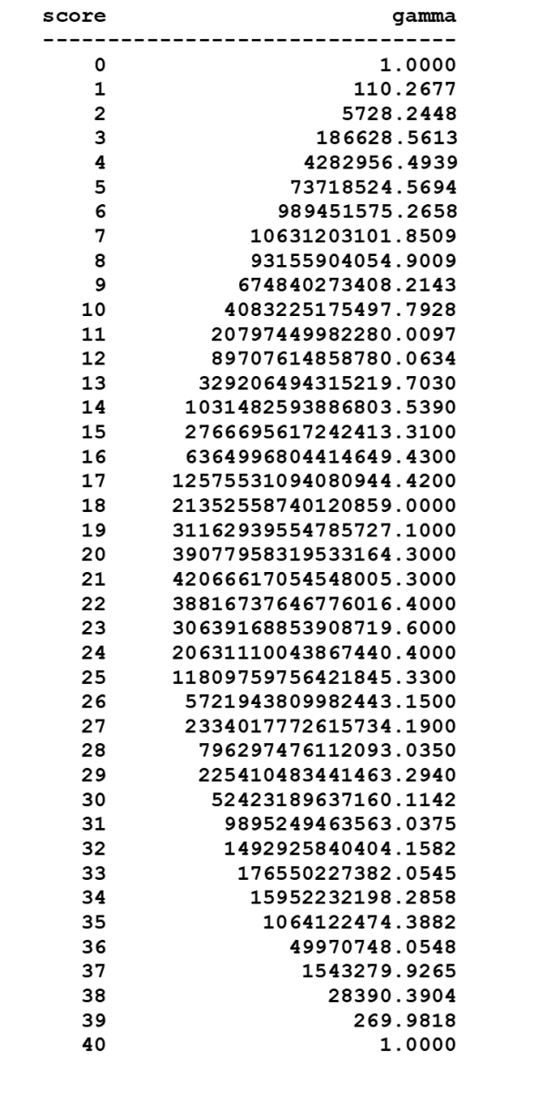
Item map
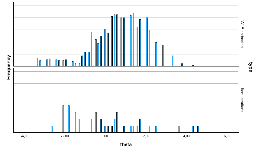
WLE Estimates
914 persons
Score Count pct cumulated WML bias sem
--------------------------------------------------
0 0 0.000 0.000 -5.425 0.491 0.648
1 3 0.003 0.003 -4.267 0.063 0.765
2 6 0.007 0.010 -3.695 0.007 0.705
3 6 0.007 0.016 -3.297 -0.001 0.629
4 7 0.008 0.024 -2.982 -0.001 0.566
5 8 0.009 0.033 -2.716 -0.001 0.520
6 7 0.008 0.040 -2.482 -0.000 0.487
7 6 0.007 0.047 -2.270 -0.000 0.463
8 6 0.007 0.054 -2.073 0.000 0.445
9 7 0.008 0.061 -1.888 0.000 0.431
10 5 0.005 0.067 -1.713 0.000 0.421
11 3 0.003 0.070 -1.544 0.000 0.412
12 3 0.003 0.073 -1.380 0.000 0.406
13 11 0.012 0.085 -1.220 0.000 0.401
14 15 0.016 0.102 -1.064 0.000 0.397
15 15 0.016 0.118 -0.909 0.000 0.394
16 20 0.022 0.140 -0.757 0.000 0.393
17 16 0.018 0.158 -0.605 0.000 0.392
18 28 0.031 0.188 -0.454 0.000 0.391
19 24 0.026 0.214 -0.302 0.000 0.392
20 32 0.035 0.249 -0.150 -0.000 0.393
21 39 0.043 0.292 0.003 -0.000 0.395
22 35 0.038 0.330 0.158 -0.000 0.398
23 52 0.057 0.387 0.316 -0.000 0.401
24 54 0.059 0.446 0.476 -0.000 0.406
25 54 0.059 0.505 0.640 0.000 0.412
26 51 0.056 0.561 0.810 0.000 0.418
27 51 0.056 0.617 0.985 0.000 0.427
28 53 0.058 0.675 1.167 0.000 0.437
29 56 0.061 0.736 1.359 0.000 0.449
30 41 0.045 0.781 1.561 0.000 0.463
31 49 0.054 0.835 1.777 0.000 0.481
32 51 0.056 0.891 2.010 0.001 0.502
33 38 0.042 0.932 2.265 0.001 0.529
34 25 0.027 0.960 2.551 0.001 0.561
35 22 0.024 0.984 2.876 0.001 0.603
36 11 0.012 0.996 3.256 -0.000 0.657
37 3 0.003 0.999 3.716 -0.003 0.729
38 1 0.001 1.000 4.286 -0.012 0.822
39 0 0.000 1.000 5.042 -0.066 0.891
40 0 0.000 1.000 6.382 -0.520 0.727
Range of persons with bias < 0.01: [-3.760 - 4.204]
Range of persons with bias < 0.05: [-4.184 - 4.913]
+--------------- --------+
| |
| Adjusted WLE estimates |
| |
+------------------------+
Adjusted estimates assessed at the values of the AML estimates.
Theta True Score
Score estimate score Bias RMSE SEM
-----------------------------------------------------------
0 -6.698 0.13 0.352 0.989 0.37
1 -3.950 1.90 -0.032 1.120 1.30
2 -3.484 2.85 0.000 0.818 1.56
3 -3.484 2.85 0.000 0.818 1.56
4 -3.024 4.16 -0.000 0.611 1.81
5 -2.597 5.74 -0.000 0.514 2.03
6 -2.499 6.15 0.000 0.498 2.08
7 -2.323 6.94 0.000 0.473 2.16
8 -2.060 8.24 -0.000 0.446 2.27
9 -1.864 9.27 0.000 0.431 2.34
10 -1.717 10.10 0.000 0.422 2.38
11 -1.557 11.02 0.000 0.413 2.43
12 -1.381 12.07 -0.000 0.406 2.47
13 -1.213 13.11 -0.000 0.401 2.50
14 -1.061 14.07 0.000 0.397 2.52
15 -0.913 15.01 0.000 0.395 2.54
16 -0.760 16.00 -0.000 0.393 2.55
17 -0.604 17.02 -0.000 0.392 2.55
18 -0.451 18.01 -0.000 0.391 2.56
19 -0.302 18.99 0.000 0.392 2.55
20 -0.153 19.96 0.000 0.393 2.55
21 0.004 20.97 0.000 0.395 2.53
22 0.159 21.96 -0.000 0.398 2.52
23 0.316 22.94 -0.000 0.401 2.49
24 0.474 23.92 -0.000 0.406 2.47
25 0.638 24.90 0.000 0.411 2.43
26 0.812 25.91 0.000 0.418 2.39
27 0.990 26.91 -0.000 0.427 2.35
28 1.165 27.86 -0.000 0.436 2.30
29 1.348 28.81 0.000 0.448 2.24
30 1.563 29.85 0.000 0.463 2.17
31 1.798 30.92 -0.000 0.483 2.09
32 2.000 31.78 -0.000 0.503 2.02
33 2.217 32.62 0.000 0.527 1.93
34 2.614 34.00 -0.000 0.579 1.78
35 2.905 34.87 -0.000 0.626 1.67
36 3.058 35.28 0.000 0.653 1.62
37 3.983 37.27 -0.002 0.855 1.32
38 4.212 37.65 -0.004 0.948 1.25
39 4.655 38.27 0.012 1.184 1.12
40 7.608 39.87 -0.368 1.047 0.36
References
Andersen, E. B. (1970). Asymptotic properties of conditional maximum-likelihood estimators. Journal of the Royal Statistical Society: Series B (Methodological), 32(2), 283–301. https://doi.org/10.1111/j.2517-6161.1970.tb00842.x
Andersen, E. B. (1972). The numerical solution of a set of conditional estimation equations. Journal of the Royal Statistical Society: Series B (Methodological), 34(1), 42–54. https://doi.org/10.1111/j.2517-6161.1972.tb00887.x
Andersen, E. B. (1973a). Conditional inference and models for measuring. Mentalhygiejnisk Forlag.
Andersen, E. B. (1973b). A goodness of fit test for the Rasch model. Psychometrika, 38(1), 123–140. https://doi.org/10.1007/BF02291180
Andersen, E. B. (1973c). Conditional inference for multiple-choice questionnaires. British Journal of Mathematical and Statistical Psychology, 26(1), 31–44. https://doi.org/10.1111/j.2044-8317.1973.tb00574.x
Andersen, E. B. (1977). Sufficient statistics and latent trait models. Psychometrika, 42(1), 69–81. https://doi.org/10.1007/BF02294044
Andrich, D. (1988). Rasch models for measurement. SAGE Publications.
Andrich, D. (2013). From the archives: A 1981 interview with Benjamin Drake Wright. Rasch Measurement Transactions, 27(3), 1427–1437.
Christensen, K. B. (2013). Estimation of item parameters. In K. B. Christensen, S. Kreiner, & M. Mesbah (Eds.), Rasch models in health (pp. 49–62). ISTE & John Wiley & Sons.
Fischer, G. H. (1995). Derivations of the Rasch model. In G. H. Fischer & I. W. Molenaar (Eds.), Rasch models: Foundations, recent developments, and applications (pp. 15–38). Springer-Verlag.
Fischer, G. H., & Molenaar, I. W. (Eds.). (1995). Rasch models: Foundations, recent developments, and applications. Springer-Verlag.
Hoijtink, H., & Boomsma, A. (1995). On person parameter estimation in the dichotomous Rasch model. In G. H. Fischer & I. W. Molenaar (Eds.), Rasch models: Foundations, recent developments, and applications (pp. 53–68). Springer-Verlag.
Kreiner, S. (2003). Introduction to DIGRAM (Research Report 03/10). Department of Biostatistics, University of Copenhagen.
Kreiner, S., & Christensen, K. B. (2013). Person parameter estimation and measurement in Rasch models. In K. B. Christensen, S. Kreiner, & M. Mesbah (Eds.), Rasch models in health (pp. 63–78). ISTE & John Wiley & Sons.
Kreiner, S., Hansen, M., & Hansen, C. R. (2006). On local homogeneity and stochastically ordered mixed Rasch models. Applied Psychological Measurement, 30(4), 271–297. https://doi.org/10.1177/0146621605283251
Kreiner, S., & Nielsen, T. (2013). Item analysis in DIGRAM: Guided tours (Research Report 13/06). Department of Biostatistics, University of Copenhagen.
Lord, F. M. (1983). Unbiased estimation of ability parameters, of their variance, and of their parallel-forms reliability. Psychometrika, 48(2), 233–245. https://doi.org/10.1007/BF02294018
Molenaar, I. W. (1995). Estimation of item parameters. In G. H. Fischer & I. W. Molenaar (Eds.), Rasch models: Foundations, recent developments, and applications (pp. 39–52). Springer-Verlag.
Rasch, G. (1960). Probabilistic models for some intelligence and attainment tests. Nielsen & Lydiche.
Rasch, G. (1961). On general laws and the meaning of measurement in psychology. In J. Neyman (Ed.), Proceedings of the Fourth Berkeley Symposium on Mathematical Statistics and Probability (Vol. 4, pp. 321–334). University of California Press.
Rasch, G. (1966). An individualistic approach to item analysis. In P. F. Lazarsfeld & N. W. Henry (Eds.), Readings in mathematical social science (pp. 89–108). Science Research Associates.
Rasch, G. (1967). An informal report on objectivity in comparisons. In Psychological measurement theory: Proceedings of the NUFFIC International Summer Session in Science at “Het Oude Hof”, The Hague, July 14–28, 1966 (pp. 321–334). Leiden.
Rasch, G. (1968). A mathematical theory of objectivity and its consequences for model construction. Paper presented at the European Meeting on Statistics, Econometrics and Management Science, Amsterdam, September 22–27, 1968.
Rasch, G. (1977). On specific objectivity: An attempt at formalizing the request for generality and validity of scientific statements. Danish Yearbook of Philosophy, 14, 58–94.
Warm, T. A. (1989). Weighted likelihood estimation of ability in item response theory. Psychometrika, 54(3), 427–450. https://doi.org/10.1007/BF02294627
Wright, B. D., & Douglas, G. A. (1977). Conditional versus unconditional procedures for sample-free item analysis. Educational and Psychological Measurement, 37(3), 573–586. https://doi.org/10.1177/001316447703700304
Wright, B. D., & Panchapakesan, N. (1969). A procedure for sample-free item analysis. Educational and Psychological Measurement, 29(1), 23–48. https://doi.org/10.1177/001316446902900102
Zwinderman, A. H. (1995). Pairwise parameter estimation in Rasch models. Applied Psychological Measurement, 19(4), 369–375. https://doi.org/10.1177/014662169501900405
Zwinderman, A. H., & Van den Wollenberg, A. L. (1990). Robustness of marginal maximum likelihood estimation in the Rasch model. Applied Psychological Measurement, 14(1), 73–81. https://doi.org/10.1177/014662169001400107
