1. Introduction

In educational tests, we expect local dependence between items that share a common stimulus material, e.g. a text passage or a graph. Likewise, in self-reported health scales measuring physical functioning, items may be locally dependent if they refer to a specific body part or action. In such situations, we refer to a subset of items as an item bundle, when there are features of items that may induce local dependence within the bundle and to models for sets of items with several locally independent bundles as bundle models. The notion of item bundles was first introduced by Rosenbaum (1988) describing local dependence issues in IRT models.

The purpose of this note is to compare measurement and fit issues of two types of generalizations of Rasch models in which local dependence is permitted. The first is the log-linear Rasch model (LLRM) of Kelderman (1984) and the second is the Rasch model for item bundles (RMB) defined by Wilson and Adams (1995). The paper shows that items fit a RMB if-and-only-if they fit a LLRM and compare measurement and analyses of fit of the two types of models. In addition to this, we will also show how to extend a seminal characterization of Rasch models in terms of sufficient person scores to a similar result for LLRMs.

Correspondence should be made to Kreiner, S, Section of Biostatistics, Department of Public Health, University of Copenhagen, Øster Farigmagsgade 5, B, 2099, Copenhagen K, Denmark. Email: svend.kreiner@mail.tele.dk

© 2026 The Authors .This is an open access article under the CC BY 4.0 license (https://creativecommons.org/licenses/by/4.0/)

1.1 Log-linear Rasch models

The LLRM describes the joint distribution of responses to k items by a log-linear model for a k-dimensional contingency table with main effects that depend on the person parameter θ and interaction parameters that do not depend on θ. We refer to Kreiner and Christensen (2007) for information on LLRMs. In LLRMs, bundle models are characterized by the following properties:

• Uniform associations between items in bundles.
• The total person score R over items is sufficient for θ.
• Conditional inference estimating main effects and interaction parameters and testing the fit of the model in the distribution of responses to items given R is possible.
• Bundle scores are distributed as polytomous items from conventional Rasch models.

In other words, the only difference between the LLRM for item bundles and the conventional Rasch model is that there is zero association between all items of the Rasch model and uniform association between items within the bundles of the LLRM.

1.2 IRT models for item bundles

Rosenbaum (1988) provided the first attempt to define IRT models for item bundle models and showed that super items defined by bundle scores over dichotomous items satisfy fundamental psychometric validity requirements, if the local dependencies among items were positive. Measurement would be unidimensional and expected scores on super items are monotonous increasing functions of the latent trait. The paper provides no information on specific types of parametric IRT models for polytomous items that satisfies these assumptions. We therefore read Rosenbaum (1988) as a paper about non-parametric IRT or Mokken models for item bundles.

1.3 Rasch models for item bundles

Wilson and Adams (1995) defined several types of bundle models for items from Rasch models. The model that we refer to as the RMB, is the same as the model that Wilson and Adams referred to as the saturated bundle model with properties that are similar to the properties of the LLRM model for item bundles. RMB has the following properties:

• The total person score R over items is sufficient for θ,
• Super items defined by the sums of item scores in the bundles are distributed as polytomous partial credit items from conventional Rasch models.
• It is possible to calculate conditional maximum likelihood (CML) estimates of the item parameters of the super items defined by bundle scores and to test the fit of the two bundle models conditionally given R in the same way as for conventional Rasch models. 

We refer to the distribution of a polytomous items in Rasch models as the partial credit distribution. The difference between the RMB and the LLRM is that the partial credit distribution is one of the assumptions that define the RMB, whereas it is derived from the log-linear association structure of the LLRM.

In both models, weighted likelihood estimates of θ provide a close to unbiased estimate of θ with standard errors that are asymptotically decreasing as the number of items increase towards infinity. However, since the two models provide the same measure in terms of the person score and use the same way to estimate the person parameter, the questions is whether the measurements provided by the models are different or whether one is better than the other.

2. Two examples

2.1 The physical functioning scale

The physical functioning (PF) subscale of the SF36 is an archetypal example of a scale needing a model for item bundles, because it is obvious that some items have to be locally dependent. Kreiner and Christensen (2007) analyzed data on the PF subscale from a Danish health survey from 1995. They used a graphical log-linear Rasch model (GLLRM), because they were concerned with both differential item functioning (DIF) and local dependence. However, we will disregard the DIF issues here and only compare item analyses by the RMB and LLRM models based on the same expectations of local dependence within item bundles. The PF items ask how much the respondent’s health limits the following ten activities:

A: Vigorous activities

B: Moderate activities

C: Lifting or carrying groceries

D: Climbing several flights of stairs

E: Climbing one flight of stairs

F: Bending, kneeling, or stooping

G: Walking more than one mile

H: Walking several blocks

I: Walking one block

J: Bathing or dressing yourself

Response categories are “Not limited”, Limited a little”, and “Limited a lot”.

The PF subscale consists of three obvious bundles, (A, B, C), (D, E), and (G, H, I). The RMB replaces the items of these bundles with three super items, X=A+B+C, Y=D+E, and Z= G+H+I. The LLRM analysis showed that there was local dependence among the items of the bundles. The initial item analysis disclosed highly significant evidence of local dependence within five pairs of items: (A, B), (B, C), (D, E), (G, H) and (H, I), but accepted hypotheses of local independence^[1] for (A, C) and (G, I).

Since we have two apparently very different bundle models, we have two issues to address. The first is whether measurement provided by the estimates of the person parameter by the two models are consistent. The second is whether tests of fit reject one or both models.

Figure 1 takes care of the consistency. It plots the two sets of person parameter estimates as Weighted Likelihood Estimates (WLE) against each other, excluding the biased estimates defined by extreme scores. The result shows that the estimates are more than consistent. They are close to identical. The difference between the LLRM and RMB estimates are less than 0.06 logits.

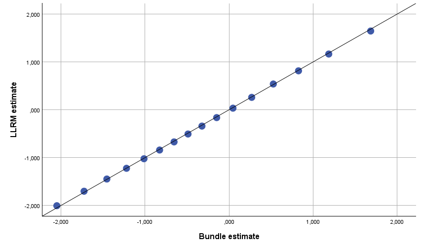
Figure 1.

 Plots of WLE estimates of θ by the RMB against the estimates of θ by the LLRM

The tests of item fit agree on where the problems are, but do not agree on what the problems are. The RMB rejects item fit of X=A+B+C and Y=D+E, whereas the LLRM rejects item A of the first bundle and item E of the second. This difference is very important. Tests of fit of the LLRM provide more concrete information on the fit issues than tests of fit of the RMB. The LLRM analysis of Kreiner and Christensen (2007) rejected item A and took care of the reason why item E was rejected in the current analysis in a way that did not imply that item E had to be rejected. The RMB had to reject both X and Y, reducing the PF scale to a summary of five items.

2.2 PIRLS

Kreiner et al. (2026) describe analyses of data from the study of Progress in International Reading and Literacy Study (PIRLS). Data consisted of responses to 32 items defined by two texts: “Mary’s Red Hen” with items M1-M16 and “The Green Turtle” with items T1-T16. Local dependencies within texts were expected. Kreiner et al. (2026) therefore fitted a LLRM to the two texts and calculated WLE of the person parameters. We refer to the paper for information on the LLRM. The dependence structure is relatively complicated. Thirteen items were locally independent and 17 pairs of two-way interactions were needed to describe the associations between the 19 locally dependent items.

Analysis by an LLRM model with 32 items is time consuming. If measurement had been the only issue, it would have been much more practical to use an RMB model with the two super items M = Σ_iM_i and T = Σ_iT_i instead of the LLRM. However, the LLRM was needed because the paper intended to illustrate criterion-referenced interpretation by estimates of scale-anchored response probabilities^[2]. Here, the issue is the same as for the PF example: do both models fit data and are the estimates by the two models consistent?

A RMB model defined by two super items is formally the same as the so-called Leunbach model defined by Leunbach (1976). Adroher et al. (2019) and Nielsen et al. (2020) present applications of test equating using the Leunbach model and assess the model’s goodness-of-fit. We have used the same methods to test the fit of the Leunbach model to the RMB model of M and T. The tests of fit comfortably accepted the RMB model. For this reason, only one issue remains. Are the estimates of person parameters from the LLRM and the RMB consistent?

Figure 2 compares the two sets of estimates. Since it is known that estimates of person parameters in Rasch models close to extreme scores may be biased, we only consider estimates defined by scores where WLE are unbiased. The differences between the two sets of estimates are larger than in the PF example, but the impression is the same. Estimates of person parameters by LLRM and RMB models are close to equivalent. Since this is the second time we find this, there is one more issue to address. There has to be a formal reason why two apparently very different models provide close to identical estimates of person parameters and agree about the fit issues. It is the main purpose of the rest of this paper to provide this explanation.

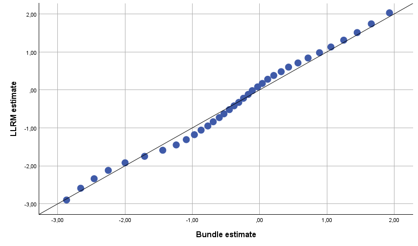
Figure 2.

Plot of RMB estimates (WLE) against LLRM estimates in the PIRLS data

3. Log-linear structure of Rasch models for item bundles

Consider first the (D, E) bundle of the PF example and the polytomous Y = D+E super item with scores from 0 to 4. It is convenient to rewrite the response distribution of a polytomous Rasch items as a power series distributions defined by a person parameter θ and a vector of item score parameters . The probabilities are 

  where                   (1)

Let  be the joint probability of responses to D and E if the person parameter is equal to θ. This means that the probability of Y = D+E is equal to

                                 (2)

To understand the relationship between the item score parameters of Y and the distribution of (D, E) it will be convenient to consider the case with θ = 0 where

 and                  (3)

In (1) we must impose identification constraints to make the item score parameters identifiable. We therefore assume that  so that (3) reduces to

                                             (4)

The p_de(0) probabilities define the distribution across the cells of a 2-dimensional contingency table which is a log-linear distribution depending on main effects and interaction effects.

                                        (5)

Therefore, inserting (5) in (4) leads to Kelderman’s log-linear Rasch model for two locally dependent items, where main effects depend on θ, and where the interaction parameter is independent of θ

                         (6)

The argument generalizes to larger item bundles, and to the complete set of items. The joint distribution of A, B, and C is a saturated log-linear Rasch model with three main effect, three two-way interactions, and a single three-way interaction. 

               (7)

During item analysis by the LLRM we test whether some of the interaction parameters are equal to zero. In our experiences with item analyses of the PF scale, we always disclose highly significant evidence of local dependence of the following pairs of items: (A, B), (B, C), (D, E), (G, H) and (H, I), but not between (A, C) and (C, I). The bundle probabilities therefore reduce to

                      (8)

                            (9)

                    (10)

Measurement by RMBs and LLRMs is consistent. Both models are log-linear Rasch models, but the LLRM is a special case of the saturated RMB that has to fit the data if the LLRM fits, because it is over-parameterized, and estimates of person parameter have to be similar. Figure 1 lives up to these expectations even though tests of fit rejected both models.

Think about an LLRM that describes a set of locally independent bundles and the corresponding saturated RMB. In such cases, evidence of misfit may turn up in three different ways. In cases where the fit of the RMB is accepted, while the fit of the LLRM is rejected, it suggests that interaction parameters are missing in the LLRM. In cases where the analysis rejects the RMB and accepts the LLRM, we have to reject the LLRM, acknowledging that our attempts to test the fit had been inadequate, overlooking evidence of either item misfit, local dependence between items from different bundles and/or or multidimensionality. In the third case, where the tests of fit rejected both models, the analysis by the LLRM may provide useful information on what the problem is and (maybe) how to correct the error, whereas the analysis by the RMB only tells us to reject one or more super items. This was what happened for the (A, B, C) bundle of the PF scale. The LLRM analysis described by Kreiner and Christensen (2007) rejected the fit of item A and accepted a model without A. An RMB analysis would have rejected all three items.

4. Characterization of log-linear Rasch models

Kreiner and Christensen (2007) did not refer to the notion of item bundles, when they decided to use a LLRM for their analysis of the PF items, but they expected that some items would be locally dependent and therefore that a conventional Rasch model could not fit the responses to PF items. Instead, they tried to fit a LLRM to data, because they knew that the LLRM shares the essential feature of the Rasch model: If the LLRM fits the data, then it follows that the total person score R is sufficient for θ, and therefore it was possible to separate inference on item properties and inference related to θ. However, there was one question that they did not ask.

The question was, whether the LLRM is the only model where R is statistically sufficient. Erling B. Andersen asked this question in his seminal paper (Andersen, 1973). His response was that the Rasch model for dichotomous model was the only model with a sufficient person score, if items were locally independent. Today, we can provide an answer to this question that extends Andersen’s characterization to a characterization of the log-linear Rasch model for dichotomous and polytomous items depending on a unidimensional person parameter: items fit a log-linear Rasch model if and only if the total score is sufficient for the person parameter.

Proving this is actually simpler than proving the RMB is a LLRM.

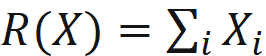To illustrate this, consider a model for k items in which the response vector X=X1,X2,…,Xk depends on a latent person parameter θ , and let R(X)=iXi denote the person’s total score. Recall that the model is discrete with a finite range RP(X) of response patterns. From this and under the assumption that R is sufficient for θ it follows that the model is a member of the family of exponential models and that the probability of a response pattern x = (x₁, x₂, … , x_k) with person score r(x) = Σ_ix_i depends on a multidimensional table L of pattern parameters,  λ(x₁, x₂, … , x_k),

                              (11)

To appreciate the role played by the pattern parameters, we once again consider the case with θ = 0 and replace the λ parameters with π(x₁, x₂, … , x_k) = exp(λ(x₁, x₂, … , x_k))

                            (12)

To make the parameters identifiable, we once again assume that .

This makes it clear that the pattern probabilities are equal to the joint probabilities of the items when θ = 0, and that we can rewrite (11) as a log-linear Rasch model with main effects that depend on θ and interaction parameters that are uniform, because they are the same at all levels of θ.

5. Parametric structure of log-linear Rasch models

To understand the different similarities of estimates of person parameters in Figures 1 and 2 we have to examine the parametric log-linear structure of the LLRM and RMB models.

5.1 The PF scale

The log-linear structure of the models for the PF scale is relatively parsimonious. A conventional Rasch model with locally independent items has only 19 parameters defined by the main effects of the items. The LLRM with five two-way interactions has 41 unknown parameters. The saturated RMB adds two-way interactions between (A, C) and (G, I) and two three-way interactions, (A, B, C) and (G, H, I), and has 60 unknown parameters. If the LLRM fits data, it therefore follows that the RMB fits an over-parameterized log-linear Rasch model to data.

5.2 PIRLS

Kreiner et al. (2026) claim that the LLRM model fits the data. Users of Rasch models who are unfamiliar with log-linear Rasch models, may regard a log-linear Rasch model for 32 items with 18 two-way interactions as a complicated model, but users of log-linear models for multidimensional contingency tables will probably regard it as a very simple model. The number of unknown parameters of a conventional Rasch model is 39, and the LLRM with a total of 18 pairs of locally dependent items has 67 unknown parameters. The RMB consisting of two super items assumes that the log-linear bundles structures are saturated and thus the RMB is over-parameterized with a total of 638,975 unknown parameters.

We do not expect over-parameterization of log-linear Rasch models to induce serious bias of estimates of person parameters, but it has to increase the standard error of the estimates. Given the amount of over-parameterizing in the RMB model, it is therefore encouraging that the differences between the LLRM and RMB estimates are not larger than what we can see in Figure 2. To underpin this assessment, Figure 3 plots the estimates of the person parameters defined by a conventional Rasch model and the LLRM against the RMB estimates in the same way as in Figure 2. It shows the measurement bias induced by application of Rasch models, where items are locally independent. Figure 3 adds the RMB estimates to the plot to make it clear the LLRM estimates are positioned very close to the RMB between the Rasch model and the RMB.

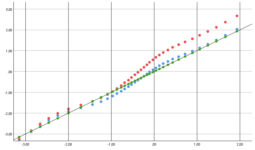
Bundle estimate

Figure 3.

Plots of estimates of person parameters by Rasch models (red) the LLRM (blue) against the estimates of the RMB (green) located at the identity line.

The shape of the curve defined by the Rasch model is similar to the shape of the curve defined by the LLRM estimates, and from this follows one additional question. Is the difference between the LLRM and RMB estimates an effect of over-parametrization of the RMB or does it reflect that something is missing in the LLRM. The tests of fit reported in Appendix A of Kreiner et al. (2026) did not reject the LLRM. However, statistically insignificant tests of fit never imply that nothing has been overlooked. It is beyond this paper to resolve this, but Figure 3 makes one important point. Comparing estimates of person parameters in Rasch or parsimonious LLRMs with estimates provided by an RMB that fits the data, may disclose evidence that there may be local dependencies that the parsimonious models have overlooked.

6. Discussion

LLRMs are versatile and practical tools providing solutions to the Rasch model’s problems with local dependence and DIF, but they are founded on very strong assumptions. Local dependencies and DIF have to be uniform in the sense that the partial or conditional associations of items have to be the same at all levels of θ. Our results show that RMBs are based on the same assumptions. Associations among items in bundles must not depend on θ. This will probably come as a useful surprise to many users of the RMB. It provides one possible reason why tests of item fit rejects a super item. The reason may be that the associations between bundle items for respondents at low levels of θ differ from the associations between bundle items at higher levels.

Item analysis by LLRMs includes a model search similar to the analysis of multidimensional contingency tables by log-linear models and may appear to be overwhelming in cases with many items. However, there is an important difference between the two types of analyses. In log-linear analyses of contingency tables with many variables we expect higher order complicated interactions and it is often time-consuming to find a model that survives all attempts to reject it. In connection with LLRMs, the starting point should be the conventional Rasch model, if we expect items to be locally independent, an RMB or a simple LLRM model, if the set of items include item bundles, or the model defined by the item screening procedure proposed by Kreiner and Christensen (2011).

Kreiner et al. (2026) did not attempt to fit an RMB model to data, but they did acknowledge that the reading test consisted of two different testlets and fitted separate LLRMs to the two testlets before they attempted to fit a joint LLRM to the data. However, in this case it would have been useful to fit the RMB before the LLRM. Our test of fit of the RMB includes comparisons of observed and expected correlations of the super items under the Leunbach model. Had the observed correlation been significantly weaker than expected, we would have concluded that the super items measure different latent traits, and would not have tried to fit a joint LLRM to the data. Had it been stronger we would have concluded that there probably were local dependence between items from the different texts. In both cases, the RMB analysis would have guided the subsequent analysis by LLRMs.   

Adroher, N.D., Kreiner, S., Young C. & Tennant A. (2019). Test equating sleep scales: applying the Leunbach model. BMC Medical Research Methodology 19, 141. https://doi.org/10.1186/s12874-019-0768-y

Andersen, E.B. (1973). Conditional inference and multiple-choice questionnaires. British Journal of Mathematical and Statistical Psychology, 26, 31–44. https://psycnet.apa.org/doi/10.1111/j.2044-8317.1973.tb00504.x

Kelderman, H. (1984). Log-linear Rasch model tests. Psychometrika, 49(2), 223–245. https://doi.org/10.1007/BF02294174

Kreiner, S., & Christensen, K. B. (2007) Validity and objectivity in health-related summated scales: Analysis by graphical log-linear Rasch models. In M. von Davier & C. H. Carstensen, Multivariate and mixture distribution Rasch models: Extensions and applications (pp. 329–346). Springer. https://doi.org/10.1007/978-0-387-49839-3_21

Kreiner, S. & Christensen, K.B.  (2011). Item screening in Graphical Log-linear Rasch models. Psychometrika, 76, 228–256. https://doi.org/10.1007/s11336-011-9203-y

Kreiner, S., Müller, M. & Nielsen, T. (2026). Criterion-referenced interpretation through scale anchoring: Illustrated by analysis of Danish results from PIRLS 2016. Educational Methods & Psychometrics, 4; 31. https://doi.org/10.83413/emp.2026.31

Leunbach, G. (1976) A probabilistic measurement model for assessing whether two tests measure the same personal factor. Technical report 1976.19. The Danish Institute of Educational Research.

Nielsen, T., Kreiner, S. & Teasdale T.W. (2020) Assessment of cognitive ability for the Danish army: Is a single score sufficient? Scandinavian Journal of Psychology, 61,161–167. https://doi.org/10.1111/sjop.12586

Rosenbaum, P.R. (1988). Item bundles. Psychometrika, 53, 349–359. https://doi.org/10.1007/BF02294217

Wilson, M., & Adams, R. J. (1995). Rasch models for item bundles. Psychometrika, 60, 181–198. https://doi.org/10.1007/BF02301412